Type function for hexagonal bin plots (a 2D analogue of a histogram). Point density is aggregated into a regular hexagonal lattice and each occupied cell is drawn as a hexagon whose fill colour encodes the number of points it contains. This is a lightweight (vectorized), pure R implementation of the canonical hexagonal binning algorithm of Carr et al. (1987).
Integer. The number of bins partitioning the range of the x-axis. Default is 30.
shape
Numeric. The aspect ratio (height/width) of the plotting region used to compute the hexagon geometry. Default is 1.
mincnt, maxcnt
Integer. Cells with counts outside the [mincnt, maxcnt] range are omitted. Defaults keep all occupied cells.
border
Colour for the hexagon borders, passed to polygon. The default NA omits the border entirely. Set a colour (e.g. “black”) for outlined hexagons. Passing the sentinel string “fill” matches the border to each cell’s fill colour, which produces perfectly seamless tiling.
fun
Function used to summarise a numericby variable within each cell (see Details). Defaults to NULL, which is equivalent to mean. Has no effect when by is absent (count mode) or discrete (modal mode).
Details
Hexagonal binning partitions the plotting region into a regular lattice of hexagons. Following the original Carr et al. (1987) algorithm, rows are spaced \(\sqrt{3}/2\) apart in scaled space, with odd rows offset by half a cell in the x-direction, while each point is assigned to its nearest lattice node.
What the fill colour encodes depends on whether a by variable is supplied (e.g. y ~ x | z):
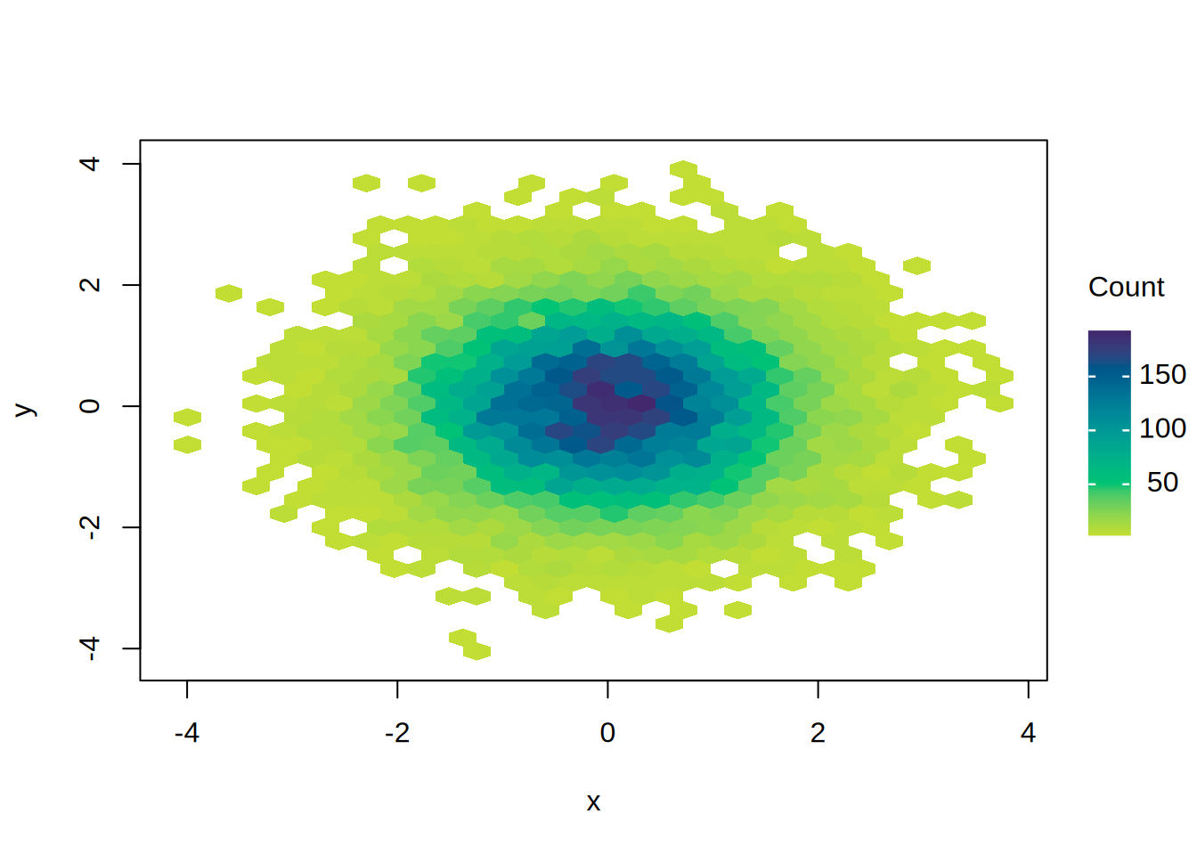
No by (default). The fill encodes the cell count, mapped to a continuous colour gradient with an automatic colourbar legend.
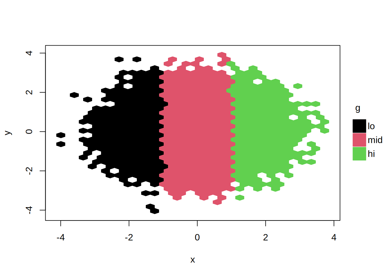
Discrete by. The fill encodes the modal (most frequent) level of the by variable within each cell, drawn with a discrete qualitative palette and legend. Useful for mapping the dominant category across a dense scatter.
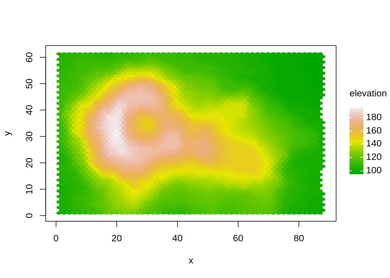
Numeric by. The fill encodes a per-cell summary of the by variable—by default the mean, or any other function passed via fun (e.g. fun = sum). Like the original no-by case, the legend is drawn as a continuous gradient. This is the hexagonal analogue of a binned heatmap.
In all three modes, the mincnt/maxcnt filters still apply to the raw cell count, so sparsely populated cells can be excluded regardless of what the colour encodes.
Because the hexagon size is derived from the data ranges, hexagons will only appear perfectly regular when the plot region’s aspect ratio matches shape. Adjust shape (or the device dimensions) if you need visually regular hexagons.
The tinyplot implementation presented here is a compact (vectorised) translation of the original Carr et al. algorithm into base R. Users requiring the fuller feature set of a dedicated hexbinning package should consult hexbin as a canonical reference, which is built on top of compiled Fortran code. Note that we have validated our cell counts against this package to confirm they match exactly.
References
Carr, D. B., Littlefield, R. J., Nicholson, W. L., and Littlefield, J. S. (1987). Scatterplot Matrix Techniques for Large N. Journal of the American Statistical Association, 82(398), 424-436. Available: https://doi.org/10.2307/2289444
Carr, D., Lewin-Koh, N., Maechler, M., and Sarkar, D. (2024). hexbin: Hexagonal Binning Routines. R package version 1.28.5. Available: https://doi.org/10.32614/CRAN.package.hexbin. The hexbin package provides the canonical implementation of this algorithm, and was a valuable reference for validating our cell counts.
Examples
library("tinyplot")set.seed(1234)dat =data.frame(x =rnorm(20000), y =rnorm(20000))# "hexbin"/"hex" type convenience stringtinyplot(y ~ x, data = dat, type ="hexbin")
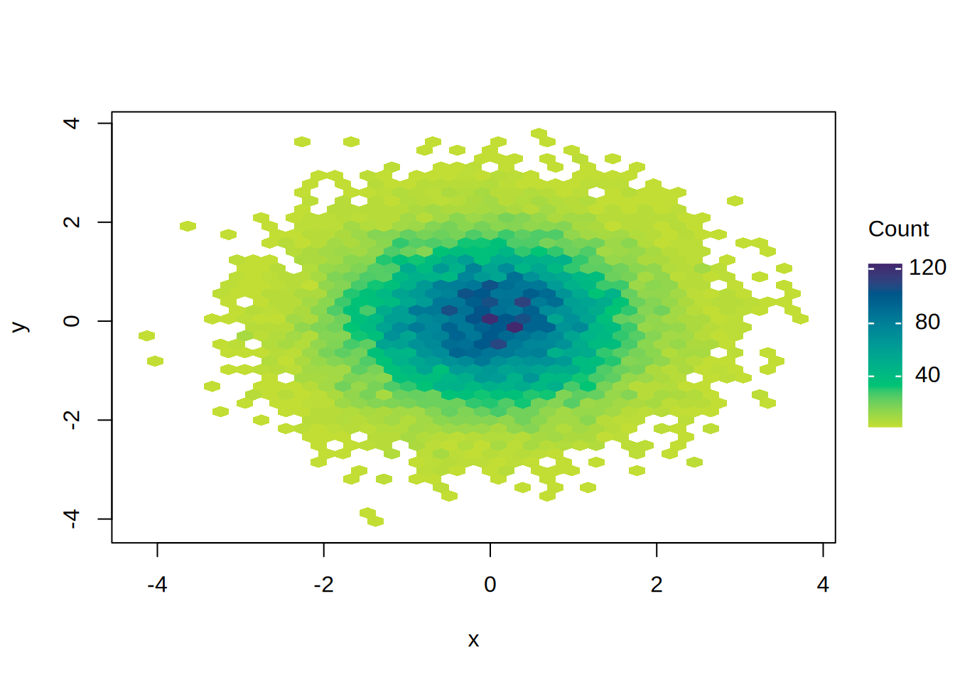
# Use type_hexbin() to pass extra argumentstinyplot(y ~ x, data = dat, type =type_hexbin(xbins =40))
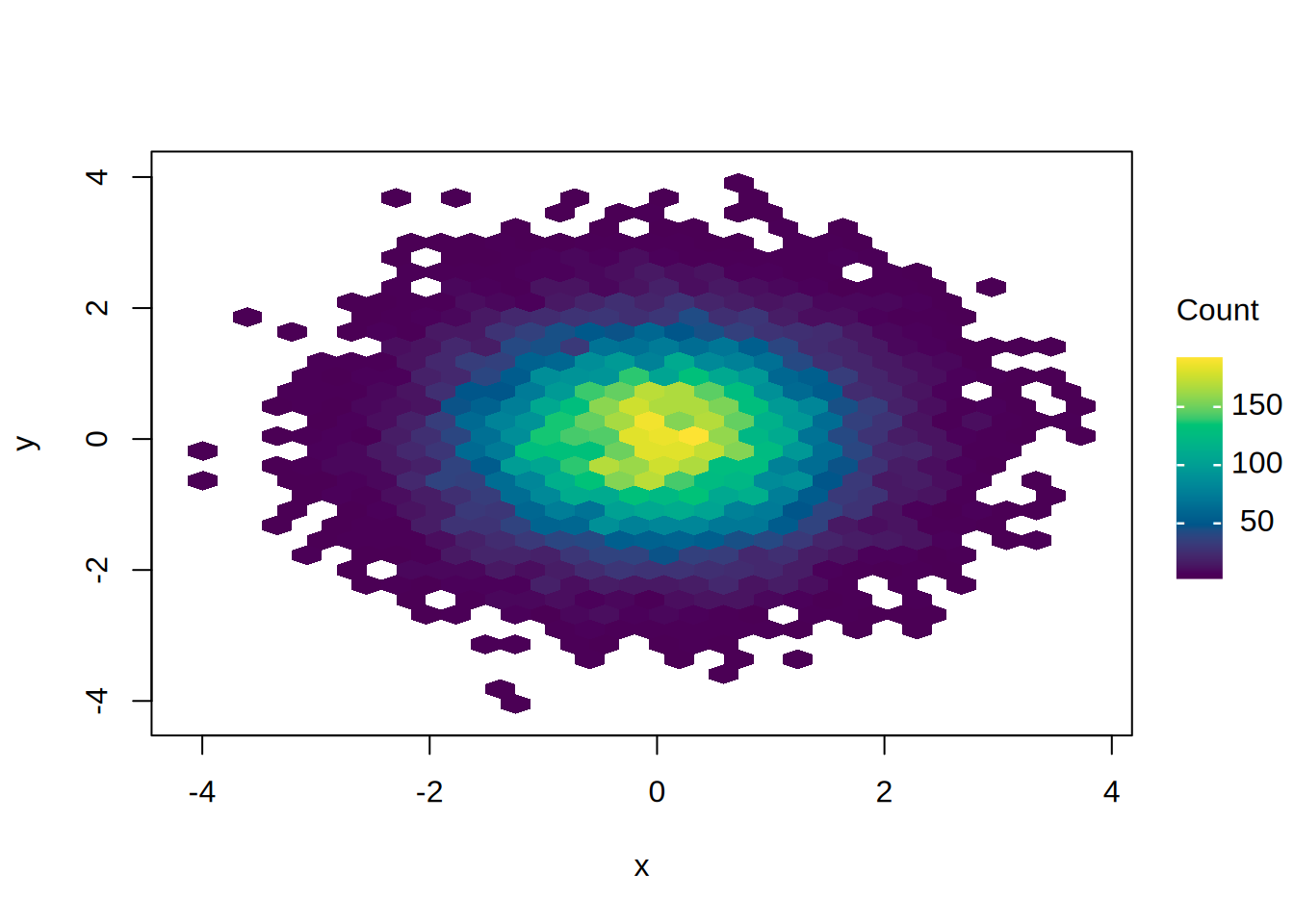
# tinyplot's default palette logic maps darker colours (the end of the# spectrum) to higher densities. For hexbin plots it can sometimes be more# visually pleasing to reverse this, which users can do manually by passing a# reversed palette.tinyplot( y ~ x, data = dat, type ="hexbin",palette =hcl.colors(100, palette ="viridis", rev =TRUE))
# Passing a `by` grouping variable will colour cells according to a summary# of this variable (in each hex cell) instead of density count. The default# summary function depends on whether `by` is discrete or continuous:# 1) Discrete grouping variable: each cell is coloured by its mode.dat$g =cut(dat$x, breaks =c(-Inf, -1, 1, Inf), labels =c("lo", "mid", "hi"))tinyplot(y ~ x | g, data = dat, type ="hexbin")
# 2) Continuous grouping variable: each cell is coloured by its mean. # Example: Create a long version of the `volcano` dataset, and plot its# elevations onto a gridded terrain map.volc =data.frame(x =as.vector(row(volcano)),y =as.vector(col(volcano)),elevation =as.vector(volcano))tinyplot( y ~ x | elevation, data = volc,type ="hexbin", xbins =50,palette =terrain.colors(100, rev =TRUE))