the smoothing bandwidth to be used, see density for details and options.
joint.bw
character string indicating whether (and how) the smoothing bandwidth should be computed from the joint data distribution when there are multiple subgroups. The options are “mean” (the default), “full”, and “none”. Also accepts a logical argument, where TRUE maps to “mean” and FALSE maps to “none”. See the "Bandwidth selection" section below for a discussion of practical considerations.
adjust
the bandwidth used is actually adjust*bw. This makes it easy to specify values like ‘half the default’ bandwidth.
kernel
a character string giving the smoothing kernel to be used. This must partially match one of “gaussian”, “rectangular”, “triangular”, “epanechnikov”, “biweight”, “cosine” or “optcosine”, with default “gaussian”, and may be abbreviated to a unique prefix (single letter).
“cosine” is smoother than “optcosine”, which is the usual ‘cosine’ kernel in the literature and almost MSE-efficient. However, “cosine” is the version used by S.
n
the number of equally spaced points at which the density is to be estimated. When n > 512, it is rounded up to a power of 2 during the calculations (as fft is used) and the final result is interpolated by approx. So it almost always makes sense to specify n as a power of two.
alpha
numeric value between 0 and 1 specifying the opacity of ribbon shading If no alpha value is provided, then will default to tpar(“ribbon.alpha”) (i.e., probably 0.2 unless this has been overridden by the user in their global settings.)
Details
The algorithm used in density.default disperses the mass of the empirical distribution function over a regular grid of at least 512 points and then uses the fast Fourier transform to convolve this approximation with a discretized version of the kernel and then uses linear approximation to evaluate the density at the specified points.
The statistical properties of a kernel are determined by \(\sigma^2_K = \int t^2 K(t) dt\) which is always \(= 1\) for our kernels (and hence the bandwidth bw is the standard deviation of the kernel) and \(R(K) = \int K^2(t) dt\). MSE-equivalent bandwidths (for different kernels) are proportional to \(\sigma_K R(K)\) which is scale invariant and for our kernels equal to \(R(K)\). This value is returned when give.Rkern = TRUE. See the examples for using exact equivalent bandwidths.
Infinite values in x are assumed to correspond to a point mass at +/-Inf and the density estimate is of the sub-density on (-Inf, +Inf).
Bandwidth selection
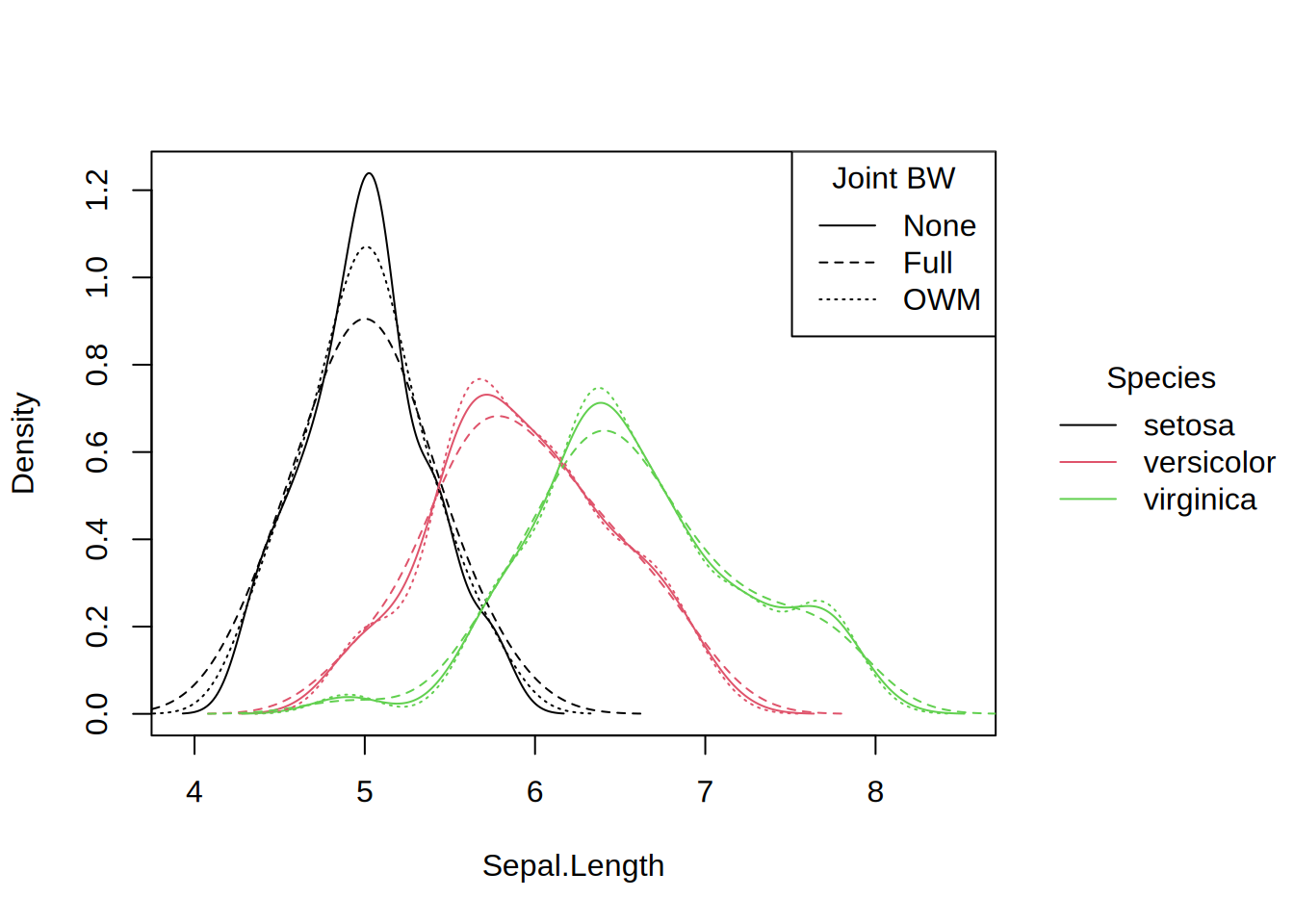
While the choice of smoothing bandwidth will always stand to affect a density visualization, it gains an added importance when multiple densities are drawn simultaneously (e.g., for subgroups with respect to by or facet). Allowing each subgroup to compute its own separate bandwidth independently offers greater flexibility in capturing the unique characteristics of each subgroup, particularly when distributions differ substantially in location and/or scale. However, this approach may overemphasize small random variations and make it harder to visually compare densities across subgroups. Hence, it is often useful to employ the same ("joint") bandwidth across all subgroups. The following strategies are available via the joint.bw argument:
The default joint.bw = “mean” first computes the individual bandwidths for each group but then computes their mean, weighted by the number of observations in each group. This will work well when all groups have similar amounts of scatter (similar variances), even when they have potentially rather different locations. The weighted averaging stabilizes potential fluctuations in the individual bandwidths, especially when some subgroups are rather small.
Alternatively, joint.bw = “full” can be used to compute the joint bandwidth from the full joint distribution (merging all groups). This will yield an even more robust bandwidth, especially when the groups overlap substantially (i.e., have similar locations and scales). However, it may lead to too large bandwidths and thus too much smoothing, especially when the locations of the groups differ substantially.
Finally, joint.bw = “none” disables the joint bandwidth so that each group just employs its individual bandwidth. This is often the best choice if the amounts of scatter differ substantially between the groups, thus necessitating different amounts of smoothing.
Titles
This tinyplot method for density plots differs from the base plot.density function in its treatment of titles. The x-axis title displays only the variable name, omitting details about the number of observations and smoothing bandwidth. Additionally, the main title is left blank by default for a cleaner appearance.
Examples
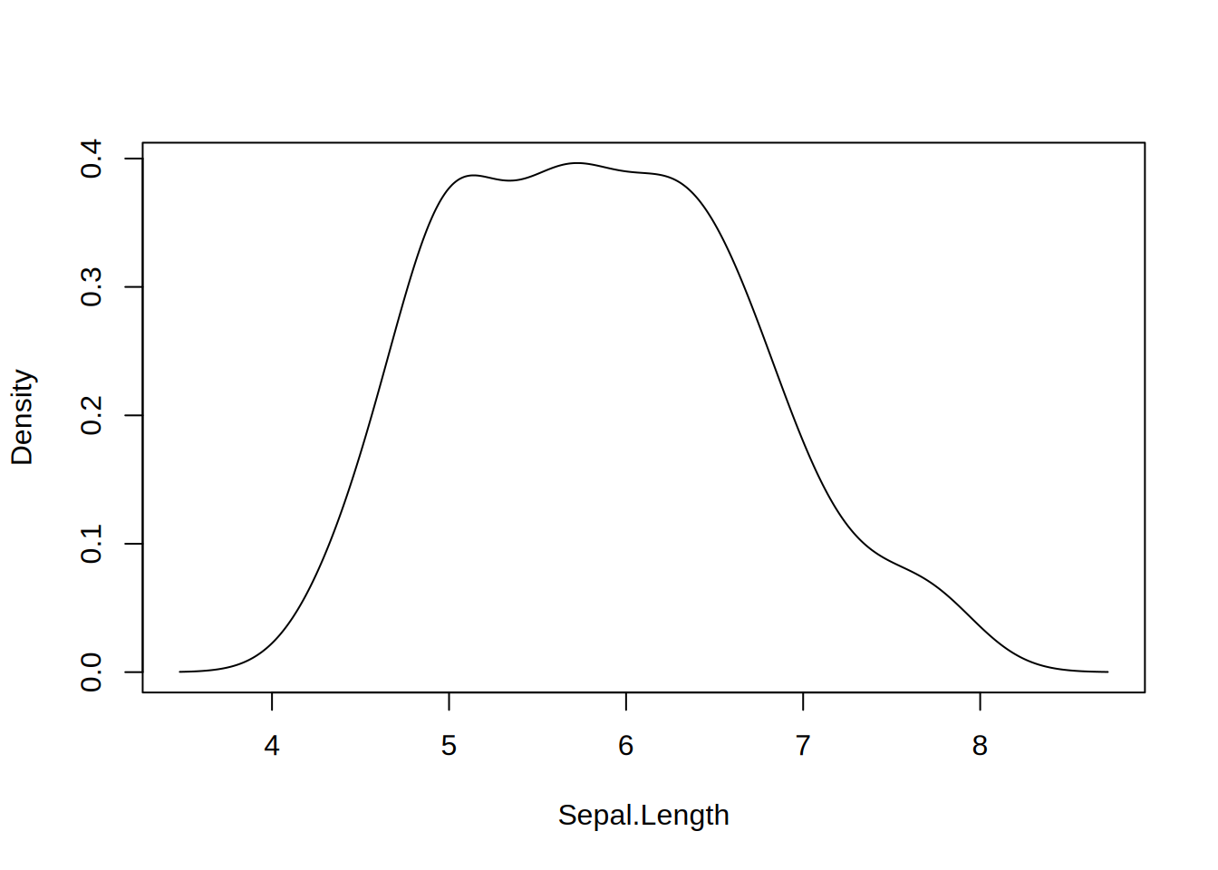
library("tinyplot")# "density" type convenience stringtinyplot(~Sepal.Length, data = iris, type ="density")
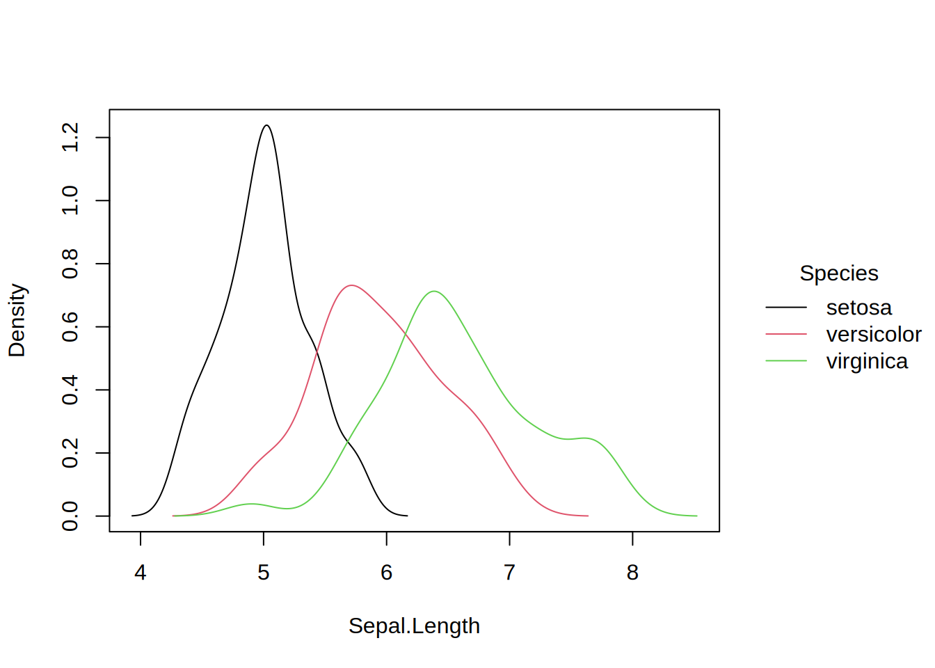
# grouped density exampletinyplot(~Sepal.Length | Species, data = iris, type ="density")
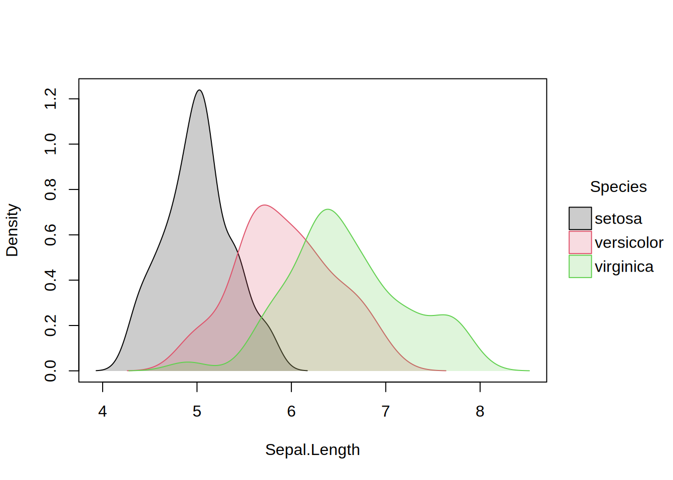
# use `bg = "by"` (or, equivalent `fill = "by"`) to get filled densitiestinyplot(~Sepal.Length | Species, data = iris, type ="density", fill ="by")
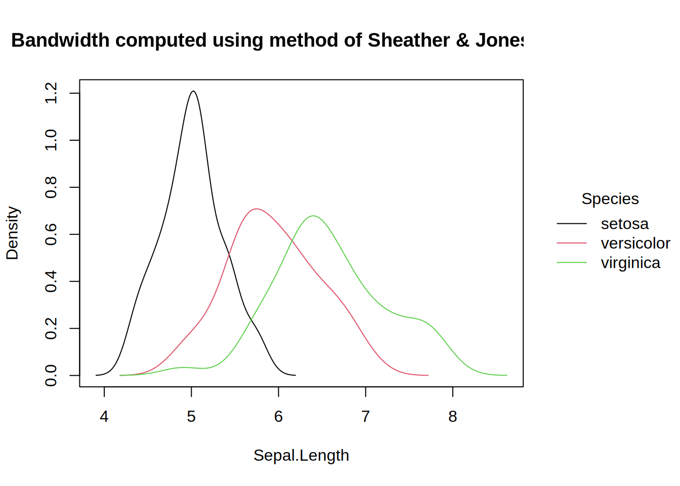
# use `type_density()` to pass extra arguments for customizationtinyplot(~Sepal.Length | Species, data = iris,type =type_density(bw ="SJ"),main ="Bandwidth computed using Sheather & Jones (1991)")
# The default for grouped density plots is to use the mean of the# individual subgroup bandwidths (weighted by group size) as the# joint bandwidth. Alternatively, the bandwidth from the "full"# data or separate individual bandwidths ("none") can be used.tinyplot(~Sepal.Length | Species, data = iris,ylim =c(0, 1.25), type ="density") # mean (default)tinyplot_add(joint.bw ="full", lty =2) # full datatinyplot_add(joint.bw ="none", lty =3) # none (individual)legend("topright", c("Mean", "Full", "None"), lty =1:3, bty ="n", title ="Joint BW")