Ribbon and area plot types

Description

Type constructor functions for producing polygon ribbons, which define a y interval (usually spanning from ymin to ymax) for each x value. Area plots are a special case of ribbon plot where ymin is set to 0 and ymax is set to y.

Usage

type_area(alpha = NULL, stack = FALSE, byord = NULL, FUN = NULL)

type_ribbon(alpha = NULL, dodge = 0, fixed.dodge = FALSE)

Arguments

alpha numeric value between 0 and 1 specifying the opacity of ribbon shading If no alpha value is provided, then will default to tpar(“ribbon.alpha”) (i.e., probably 0.2 unless this has been overridden by the user in their global settings.)
stack logical. Should the by groups be stacked on top of one another, rather than overplotted from a common zero baseline? Only relevant for grouped area plots. Default is FALSE. See the "Stacked area plots" section below.
byord

keyword string or function. Permits on-the-fly (re)ordering of the by group layers, thus controlling the order in which they stack. Options are:

  • “desc” and “asc” rank the groups by their summed y across the x axis, largest or smallest first. With “desc” the biggest group is stacked first, as the bottom layer. (Long forms like “descending” and “increasing” are also accepted.)

  • “start” and “end” instead rank on the y values at the smallest and largest x respectively, again stacking the largest group first.

  • “minvar” ranks by variance, putting the lowest variance group on the baseline.

  • “asis” or “rev” permute the existing levels without consulting the data at all. The former takes the groups in the order that they appear in the data, while the latter reverses the current level order.

  • a custom function that determines both the ranking statistic and its direction. The statistic is always sorted ascending, so function(y) -median(y) layers by median y value, from the biggest to the smallest. Note that if a function requires access to a group’s x values, then one of its arguments must be named x, e.g. function(y, x) coef(lm(y ~ x))[2] would layer by trend.

Defaults to NULL, i.e. keep the existing factor levels. To set that order explicitly, call factor(levels = …) on the grouping variable beforehand. See Examples, as well as the "Stacked area plots" section below.
FUN a function for collapsing repeated y values within a group and x position, used only when stack = TRUE. Defaults to mean, matching type_barplot(), so that the same data stacks to the same heights whether it is drawn as bars or as an area.
dodge

Adjustment parameter for dodging overlapping points or ranges in grouped plots along the x-axis (or y-axis for flipped plots). Either:

  • numeric value in the range [0,1). Note that values are scaled relative to the spacing of x-axis breaks, e.g. dodge = 0.1 places the outermost groups one-tenth of the way to adjacent breaks, dodge = 0.5 places them midway between breaks, etc. Values < 0.5 are recommended.

  • logical. If TRUE, the dodge width is calculated automatically based on the number of groups (0.1 per group for 2-4 groups, 0.45 for 5+ groups). If FALSE or 0, no dodging is performed.

Default value is 0 (no dodging). While we do not check, it is strongly recommended that dodging only be used in cases where the x-axis comprises a limited number of discrete breaks.
fixed.dodge Logical. If FALSE (default), dodge positions are calculated independently for each x value, based only on the groups present at that position. If TRUE, dodge positions are based on all groups, ensuring "fixed" spacing across x-axis breaks (i.e., even if some groups are missing for a particular x value).

Dodging ribbon plots

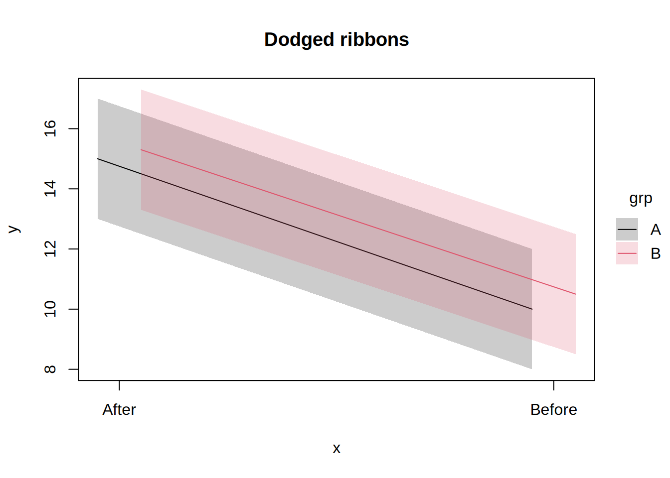
We support dodging for grouped ribbon plots, enabling similar functionality to dodged errorbar and pointrange plots. However, it is strongly recommended that dodging is only implemented for cases where the x-axis comprises a limited number of discrete cases (e.g., coefficient or event-study plots). See Examples.

Stacked area plots

Passing type_area(stack = TRUE) stacks the by groups cumulatively, rather than drawing each one from a zero baseline. Groups are accumulated in the order of their (factor) levels, so the first level forms the bottom band and the top of the final band traces the group total. Stacking is computed separately within each facet.

The byord argument is a helpful companion to stacked area plots, since it enables on-the-fly adjustment of the stacking order. For example, the size keywords—“desc”, “start”, and “end”—rank the stacked by groups according to their y values, either summed across the x axis or taken at one end of it. Following convention, the ranking runs in descending order, so that the biggest group is drawn on the bottom layer (use “asc” for the reverse). However, size is not the only route to a stable baseline. Because each band is drawn on top of the ones below it, they all inherit whatever movement the bottom layer has. A large but volatile group can therefore be a worse choice of foundation than a small, steady one. In this latter case, the “minvar” keyword would be a more appropriate choice since it places the lowest variance group at the bottom. Your choice of stacking ordering should therefore respond to the patterns in your data and which layers you want to emphasize.

Stacking needs exactly one y value per group per x value. Repeated cells —typically caused by a variable that is present in the data but absent from the plot—are collapsed with FUN (default mean) rather than being stacked against each other. Conversely, groups that are missing an x value (or have an NA there) count as contributing zero at that point, so that a gap in one group does not shift the groups stacked above it. Note that stacking negative values is not meaningful and will produce overlapping bands. Note that the legend key for stacked area plots is deliberately inverted compared to other plot types (including non-stacked area plots) to ensure a consistent ordering with the "bottoms-up" layering of the stacked regions. Similarly, reordering of the by group levels will reassign the palette, since group colours are allocated by level position. This matches what releveling a factor does elsewhere, but it does mean that reordering the bands repaints them.

Finally, note that unlike non-stacked area plots, the stacked bands are drawn with opaque fill by default, since they do not overlap. Pass an explicit alpha or fill value to override.

Examples

library("tinyplot")

x = 1:100 / 10
y = sin(x)

#
## Ribbon plots

# "ribbon" convenience string
tinyplot(x = x, ymin = y - 1, ymax = y + 1, type = "ribbon")

# Same result with type_ribbon()
tinyplot(x = x, ymin = y-1, ymax = y+1, type = type_ribbon())

# y will be added as a line if it is specified
tinyplot(x = x, y = y, ymin = y-1, ymax = y+1, type = "ribbon")

#
## Area plots

# "area" type convenience string
tinyplot(x, y, type = "area")

# Same result with type_area()
tinyplot(x, y, type = type_area())

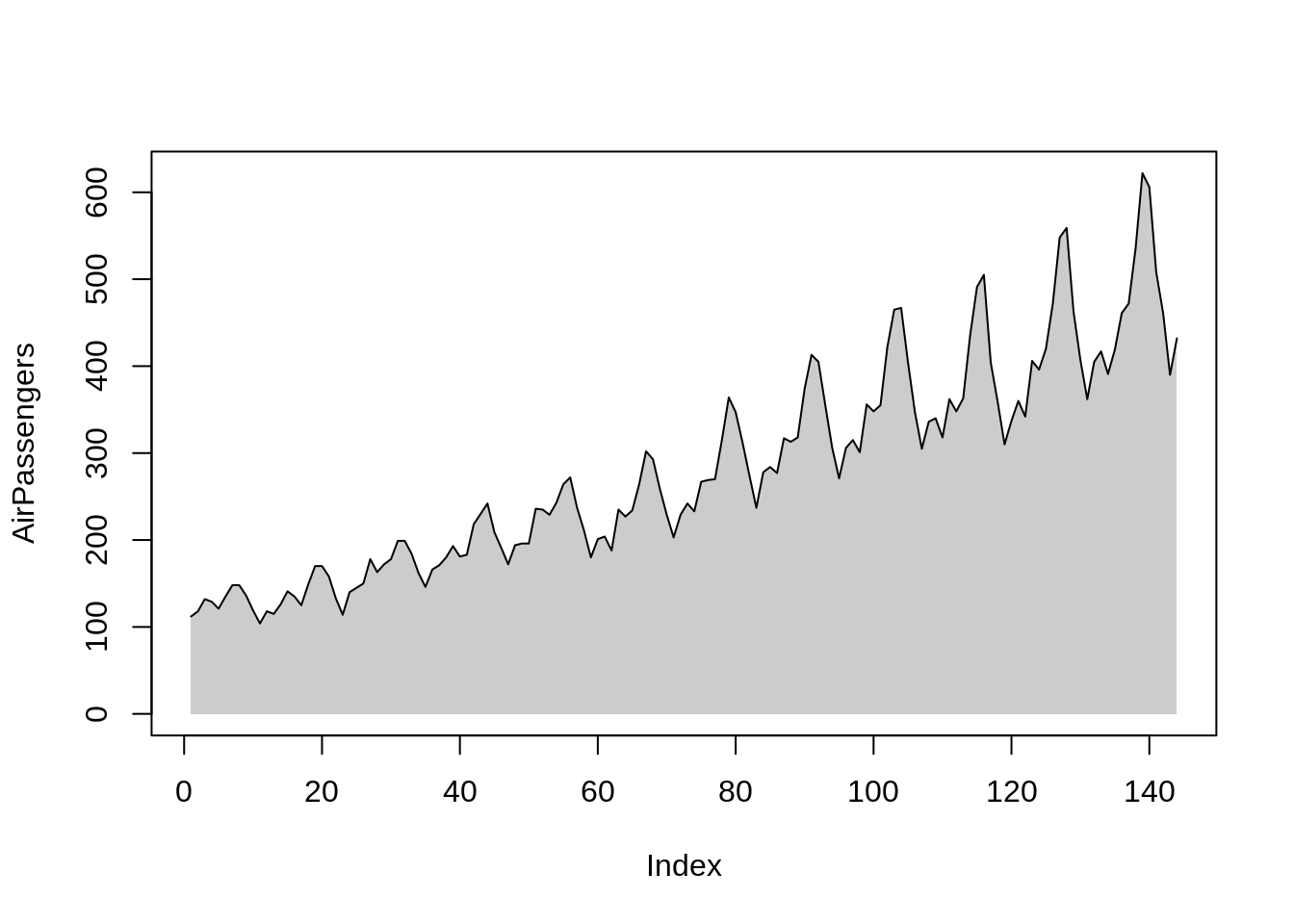
# Area plots are often used for time series charts
tinyplot(AirPassengers, type = "area")

#
## Stacked area plots

# Grouped area plots can be stacked cumulatively, rather than being drawn
# from a common zero baseline.

# Group B is small and steady; A and C are larger and wobblier.
dat = expand.grid(year = 2000:2020, grp = factor(c("A", "B", "C")))
dat$val = as.integer(dat$grp) +
  c(1.2, 0.1, 1.8)[dat$grp] * sin(dat$year / 3) +
  c(0.06, 0.02, 0.10)[dat$grp] * (dat$year - 2000)

tinyplot(val ~ year | grp, data = dat, type = type_area(stack = TRUE))

# Use `byord` to control which group stacks where. Here we stack by their
# largest end value.

tinyplot(
  val ~ year | grp, data = dat,
  type = type_area(stack = TRUE, byord = "end")
)

# `"minvar"` instead puts the *least variable* group on the baseline. Every
# band inherits the movement of the ones below it, so a steady bottom layer
# keeps the whole chart legible. Here that picks group B, which the default
# level order leaves in the middle and `"end"`/`"desc"` push to the top.

tinyplot(
  val ~ year | grp, data = dat,
  type = type_area(stack = TRUE, byord = "minvar")
)

# `"rev"` simply flips the existing level order, which is the one thing a
# ranking function cannot do (it never sees which group it was handed).

tinyplot(
  val ~ year | grp, data = dat,
  type = type_area(stack = TRUE, byord = "rev")
)

# Custom ranking functions are also accepted. Name an argument `x` and it
# receives the group's x values too, which is what a slope needs.

tinyplot(
  val ~ year | grp, data = dat,
  type = type_area(stack = TRUE, byord = function(y, x) coef(lm(y ~ x))[2])
)

# Stacking expects a single `y` value per group per `x` value. Any repeats
# are collapsed for us first, using `FUN` (`mean` by default). Here, for
# instance, ChickWeight records many chicks per diet at each timepoint.

tinyplot(
  weight ~ Time | Diet, data = ChickWeight,
  type = type_area(stack = TRUE, FUN = median)
)

# (Illustrative purposes aside, we leave it to the reader to decide whether
# stacking separate diets on top of one another makes any sense...)

#
## Dodged ribbon/area plots

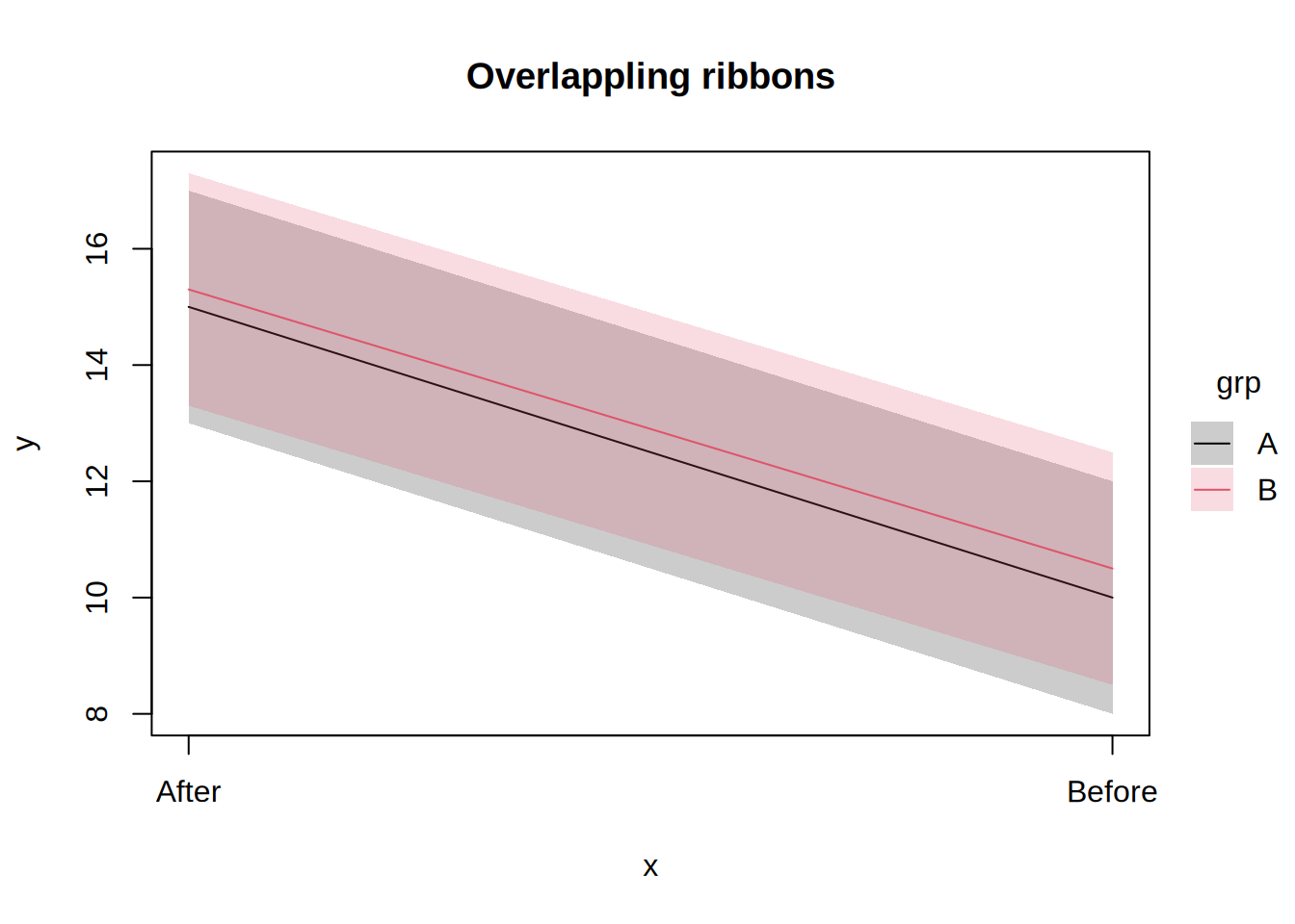
# Dodged ribbon or area plots can be useful in cases where there is strong
# overlap across groups (and a limited number of discrete x-axis values).

dat = data.frame(
  x = rep(c("Before", "After"), each = 2),
  grp = rep(c("A", "B"), 2),
  y = c(10, 10.5, 15, 15.3),
  lwr = c(8, 8.5, 13, 13.3),
  upr = c(12, 12.5, 17, 17.3)
)

tinyplot(
  y ~ x | grp,
  data = dat,
  ymin = lwr, ymax = upr,
  type = type_ribbon(),
  main = "Overlappling ribbons"
)

tinyplot(
  y ~ x | grp,
  data = dat,
  ymin = lwr, ymax = upr,
  type = type_ribbon(dodge = 0.1),
  main = "Dodged ribbons"
)