Type function for producing ridge plots (also known as joy plots), which display density distributions for multiple groups with vertical offsets. This function uses tinyplot scaffolding, which enables added functionality such as grouping and faceting.
The line color is controlled by the col argument in the tinyplot() call. The fill color is controlled by the bg argument in the tinyplot() call.
Numeric. Controls the scaling factor of each plot. Values greater than 1 means that plots overlap.
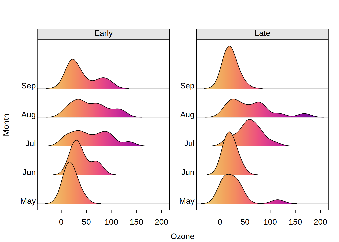
joint.max
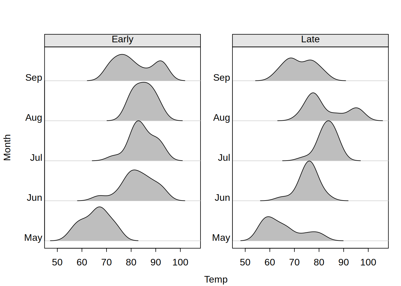
character indicating how to scale the maximum of the densities: The default “all” indicates that all densities are scaled jointly relative to the same maximum so that the areas of all densities are comparable. Alternatively, “facet” indicates that the maximum is computed within each facet so that the areas of the densities are comparable within each facet but not necessarily across facets. Finally, “by” indicates that each row (in each facet) is scaled separately, so that the areas of the densities for by groups in the same row are comparable but not necessarily across rows.
breaks
Numeric. If a color gradient is used for shading, the breaks between the colors can be modified. The default is to use equidistant breaks spanning the range of the x variable.
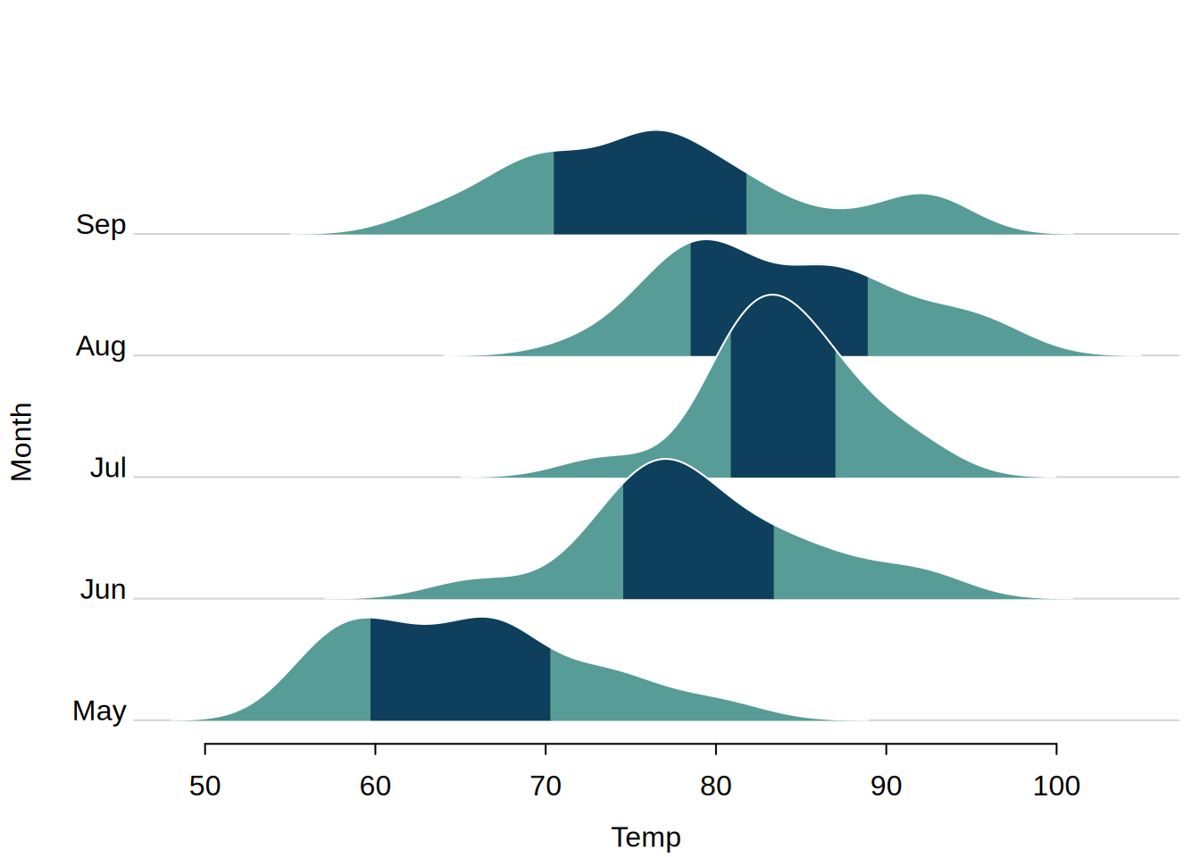
probs
Numeric. Instead of specifying the same breaks on the x-axis for all groups, it is possible to specify group-specific quantiles at the specified probs. The quantiles are computed based on the density (rather than the raw original variable). Only one of breaks or probs must be specified.
ylevels
a character or numeric vector specifying in which order the levels of the y-variable should be plotted.
bw
the smoothing bandwidth to be used. The kernels are scaled such that this is the standard deviation of the smoothing kernel. (Note this differs from the reference books cited below.)
bw can also be a character string giving a rule to choose the bandwidth. See bw.nrd. The default, “nrd0”, has remained the default for historical and compatibility reasons, rather than as a general recommendation, where e.g., “SJ” would rather fit, see also Venables and Ripley (2002).
The specified (or computed) value of bw is multiplied by adjust.
joint.bw
character string indicating whether (and how) the smoothing bandwidth should be computed from the joint data distribution. The default of “mean” will compute the joint bandwidth as the mean of the individual subgroup bandwidths (weighted by their number of observations). Choosing “full” will result in a joint bandwidth computed from the full distribution (merging all subgroups). For “none” the individual bandwidth will be computed independently for each subgroup. Also accepts a logical argument, where TRUE maps to “mean” and FALSE maps to “none”. See type_density for some discussion of practical considerations.
adjust
the bandwidth used is actually adjust*bw. This makes it easy to specify values like ‘half the default’ bandwidth.
kernel
a character string giving the smoothing kernel to be used. This must partially match one of “gaussian”, “rectangular”, “triangular”, “epanechnikov”, “biweight”, “cosine” or “optcosine”, with default “gaussian”, and may be abbreviated to a unique prefix (single letter).
“cosine” is smoother than “optcosine”, which is the usual ‘cosine’ kernel in the literature and almost MSE-efficient. However, “cosine” is the version used by S.
n
the number of equally spaced points at which the density is to be estimated. When n > 512, it is rounded up to a power of 2 during the calculations (as fft is used) and the final result is interpolated by approx. So it almost always makes sense to specify n as a power of two.
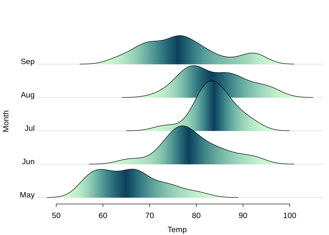
gradient
Logical or character. Should a gradient fill be used to shade the area under the density? If a character specification is used, then it can either be of length 1 and specify the palette to be used with gradient = TRUE corresponding to gradient = “viridis”. If a character vector of length greater than 1 is used, then it should specify the colors in the palette, e.g., gradient = hcl.colors(512).
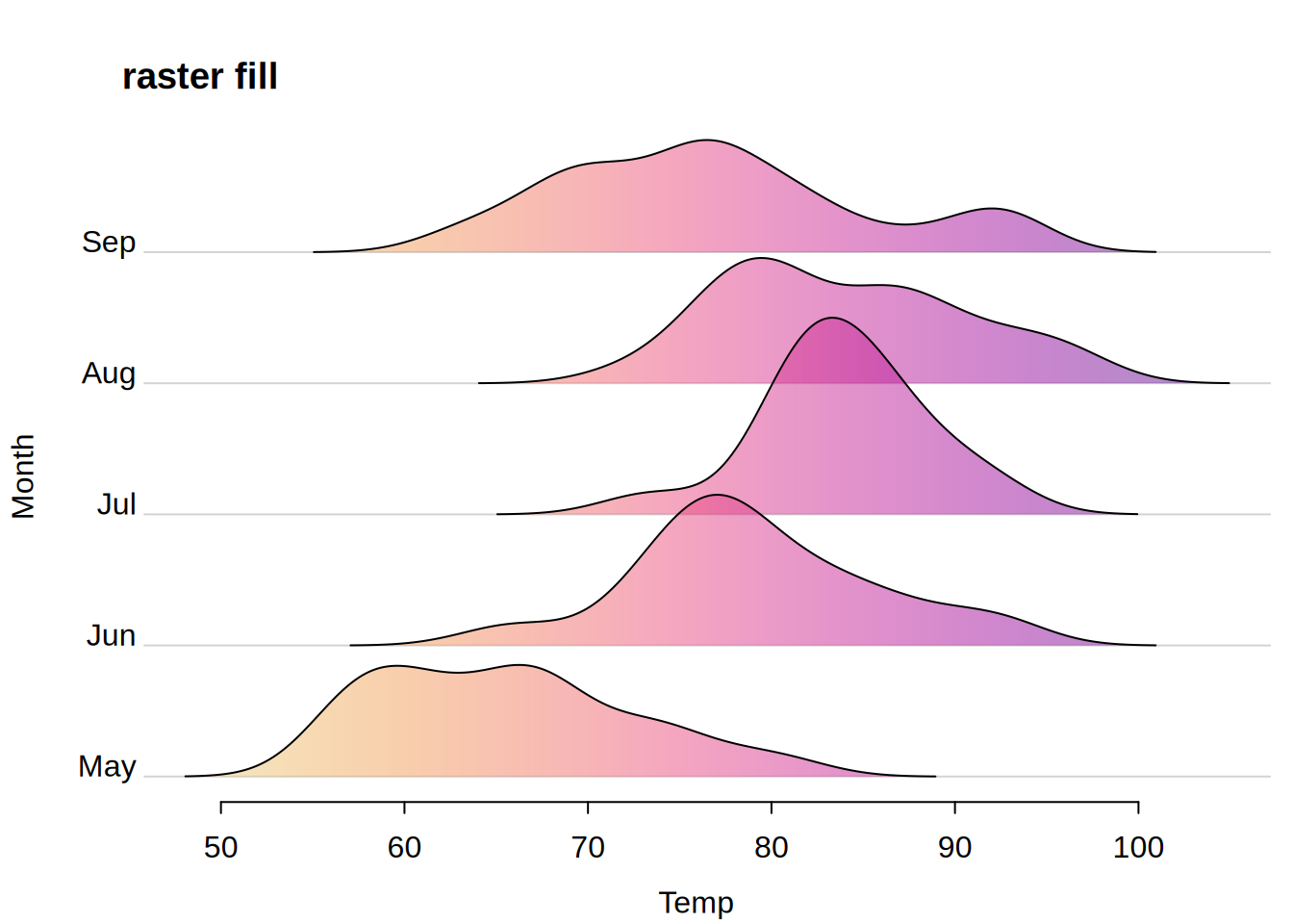
raster
Logical. Should the gradient fill be drawn using rasterImage? Defaults to FALSE, in which case the gradient fill will instead be drawn using polygon. See the Technical note on gradient fills section below.
col
Character string denoting the outline (border) color for all of the ridge densities. Note that a singular value is expected; if multiple colors are provided then only the first will be used. This argument is mostly useful for the aesthetic effect of drawing a common outline color in combination with gradient fills. See Examples.
alpha
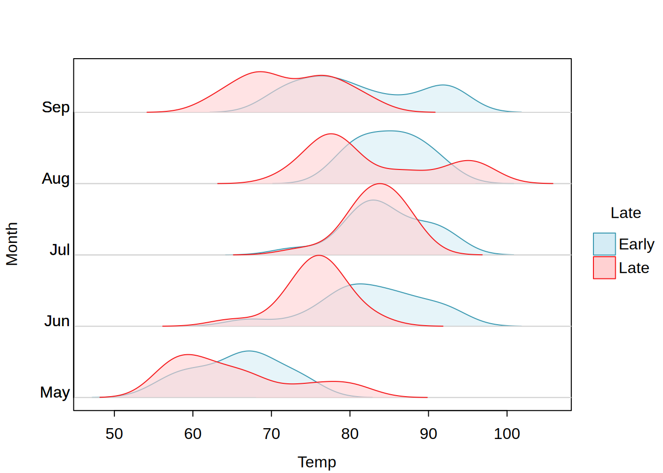
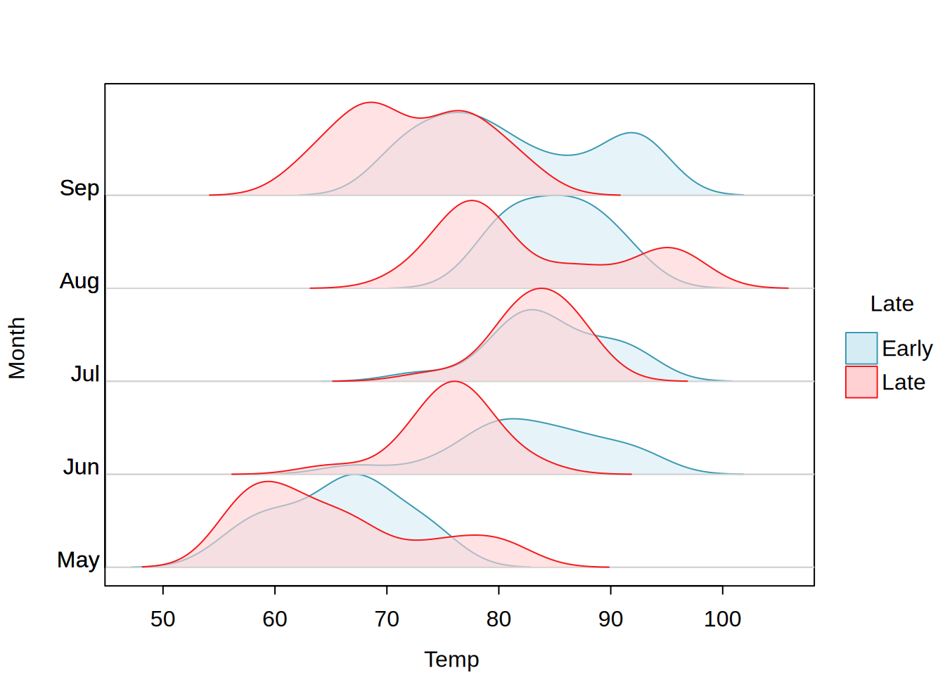
Numeric in the range [0,1] for adjusting the alpha transparency of the density fills. In most cases, will default to a value of 1, i.e. fully opaque. But for some by grouped plots (excepting the special cases where by==y or by==x), will default to 0.6.
Technical note on gradient fills
tinyplot uses two basic approaches for drawing gradient fills in ridge line plots, e.g., if type_ridge(gradient = TRUE).
The first (and default) polygon-based approach involves dividing up the main density region into many smaller polygons along the x-axis. Each of these smaller polygons inherits a different color "segment" from the underlying palette swatch, which in turn creates the effect of a continuous gradient when they are all plotted together. Internally, this polygon-based approach is vectorized (i.e., all of the sub-polygons are plotted simultaneously). It is thus efficient from a plotting perspective and generally also performs well from an aesthetic perspective. However, it can occasionally produce undesirable plotting artifacts on some graphics devices—e.g., thin but visible vertical lines—if alpha transparency is being used at the same time.
For this reason, we also offer an alternative raster-based approach for gradient fills that users can invoke via type_ridge(gradient = TRUE, raster = TRUE). The essential idea is that we coerce the density polygon into a raster representation (using rasterImage) and achieve the gradient effect via color interpolation. The trade-off this time is potential smoothness artifacts around the top of the ridge densities at high resolutions, since we have converted a vector object into a raster object.
Again, we expect that the choice between these two approaches will only matter for ridge plots that combine gradient fills with alpha transparency (and on certain graphics devices). We recommend that users experiment to determine which approach is optimal for their device.
# for ridge plots, we recommend pairing with the dedicated theme(s), which# facilitate nicer y-axis labels, grid lines, etc.tinytheme("ridge")tinyplot(Month ~ Temp, data = aq, type ="ridge")
tinytheme("ridge2") # removes the plot frame (but keeps x-axis line)tinyplot(Month ~ Temp, data = aq, type ="ridge")
# the "ridge(2)" themes are especially helpful for long y labels, due to# dyanmic plot adjustmenttinyplot(Month2 ~ Temp, data = aq, type ="ridge")
# pass customization arguments through type_ridge()... for example, use# the scale argument to change/avoid overlap of densities (more on scaling# further below)tinyplot(Month ~ Temp, data = aq, type =type_ridge(scale =1))
## by grouping is also supported. two special cases of interest:# 1) by == y (color by y groups)tinyplot(Month ~ Temp | Month, data = aq, type ="ridge")
# 2) by == x (gradient coloring along x)tinyplot(Month ~ Temp | Temp, data = aq, type ="ridge")
# aside: pass explicit `type_ridge(col = <col>)` arg to set a different# border colortinyplot(Month ~ Temp | Temp, data = aq, type =type_ridge(col ="white"))
# gradient coloring along the x-axis can also be invoked manually without# a legend (the next two tinyplot calls are equivalent)# tinyplot(Month ~ Temp, data = aq, type = type_ridge(gradient = "agsunset"))tinyplot(Month ~ Temp, data = aq, type =type_ridge(gradient =TRUE))
# aside: when combining gradient fill with alpha transparency, it may be# better to use the raster-based approach (test on your graphics device)tinyplot(Month ~ Temp, data = aq,type =type_ridge(gradient =TRUE, alpha =0.5),main ="polygon fill (default)")
# highlighting only the center 50% of the density (i.e., 25%-75% quantiles)tinyplot(Month ~ Temp, data = aq, type =type_ridge(gradient =hcl.colors(3, "Dark Mint")[c(2, 1, 2)],probs =c(0.25, 0.75), col ="white"))
# highlighting the probability distribution by color gradient# (darkest point = median)tinyplot(Month ~ Temp, data = aq, type =type_ridge(gradient =hcl.colors(250, "Dark Mint")[c(250:1, 1:250)],probs =0:500/500))
# faceting also works, although we recommend switching (back) to the "ridge"# theme for faceted ridge plotstinytheme("ridge")tinyplot(Month ~ Ozone, facet =~ Late, data = aq,type =type_ridge(gradient =TRUE))
## use the joint.max argument to vary the maximum density used for## determining relative scaling...# jointly across all densities (default) vs. per facettinyplot(Month ~ Temp, facet =~ Late, data = aq,type =type_ridge(scale =1))