Spineplot and spinogram types

Description

Type function(s) for producing spineplots and spinograms, which are modified versions of histograms or mosaic plots, and particularly useful for visualizing factor variables. Note that tinyplot defaults to type_spineplot() if y is a factor variable.

Usage

type_spineplot(
  breaks = NULL,
  tol.ylab = 0.05,
  off = NULL,
  xlevels = NULL,
  ylevels = NULL,
  col = NULL,
  xaxlabels = NULL,
  yaxlabels = NULL,
  weights = NULL,
  lighten = FALSE
)

Arguments

breaks	if the explanatory variable is numeric, this controls how it is discretized. breaks is passed to hist and can be a list of arguments.
tol.ylab	convenience tolerance parameter for y-axis annotation. If the distance between two labels drops under this threshold, they are plotted equidistantly.
off	vertical offset between the bars (in per cent). It is fixed to 0 for spinograms and defaults to 2 for spine plots.
xlevels, ylevels	a character or numeric vector specifying the ordering of the levels of the x and y variables (if character) or the corresponding indexes (if numeric) for the plot.
col	a vector of fill colors of the same length as levels(y). The default is to call gray.colors.
xaxlabels, yaxlabels	character vectors for annotation of x and y axis. Default to levels(y) and levels(x), respectively for the spine plot. For xaxlabels in the spinogram, the breaks are used.
weights	numeric. A vector of frequency weights for each observation in the data. If NULL all weights are implicitly assumed to be 1. If x is already a 2-way table, the weights are ignored.
lighten	logical. For grouped spineplots where the y variable is itself the grouping variable (i.e. y == by), should the fills use a lighter, opaque tint of the series colour(s)? Default is FALSE, i.e. the fills use the fully-saturated palette colour(s). (Unlike the other area types such as type_barplot, where lightening is the default, spineplot tiles abut one another with no gap, so the darker saturated fills read better against their matching border colours.) Set to TRUE to opt in to the lighter tint. Note that lighten has no effect on other spineplot displays (single-group or x == by), which always use a sequential shading ramp of the base colour.

Examples

library("tinyplot")

# "spineplot" type convenience string
tinyplot(Species ~ Sepal.Width, data = iris, type = "spineplot")

# Aside: specifying the type is redundant for this example, since tinyplot()
# defaults to "spineplot" if y is a factor (just like base plot).
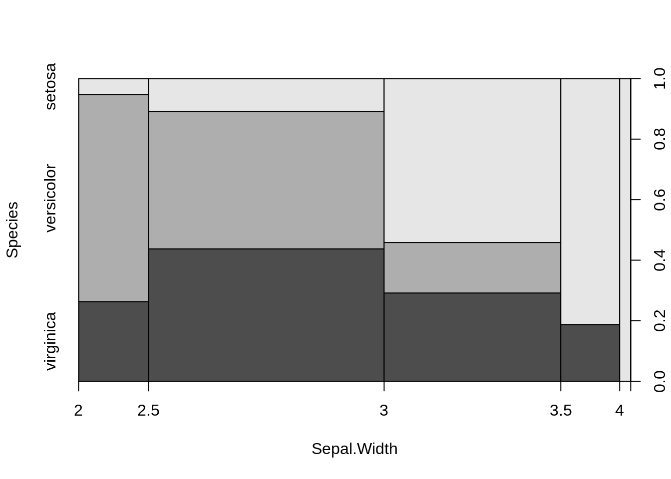
tinyplot(Species ~ Sepal.Width, data = iris)

# Use `type_spineplot()` to pass extra arguments for customization
tinyplot(
  Species ~ Sepal.Width, data = iris,
  type = type_spineplot(breaks = 4)
)

# Passing custom colors to the y-axis categories
tinyplot(
  Species ~ Sepal.Width, data = iris,
  type = type_spineplot(breaks = 4, col = palette.colors(3, "Pastel 1"))
)

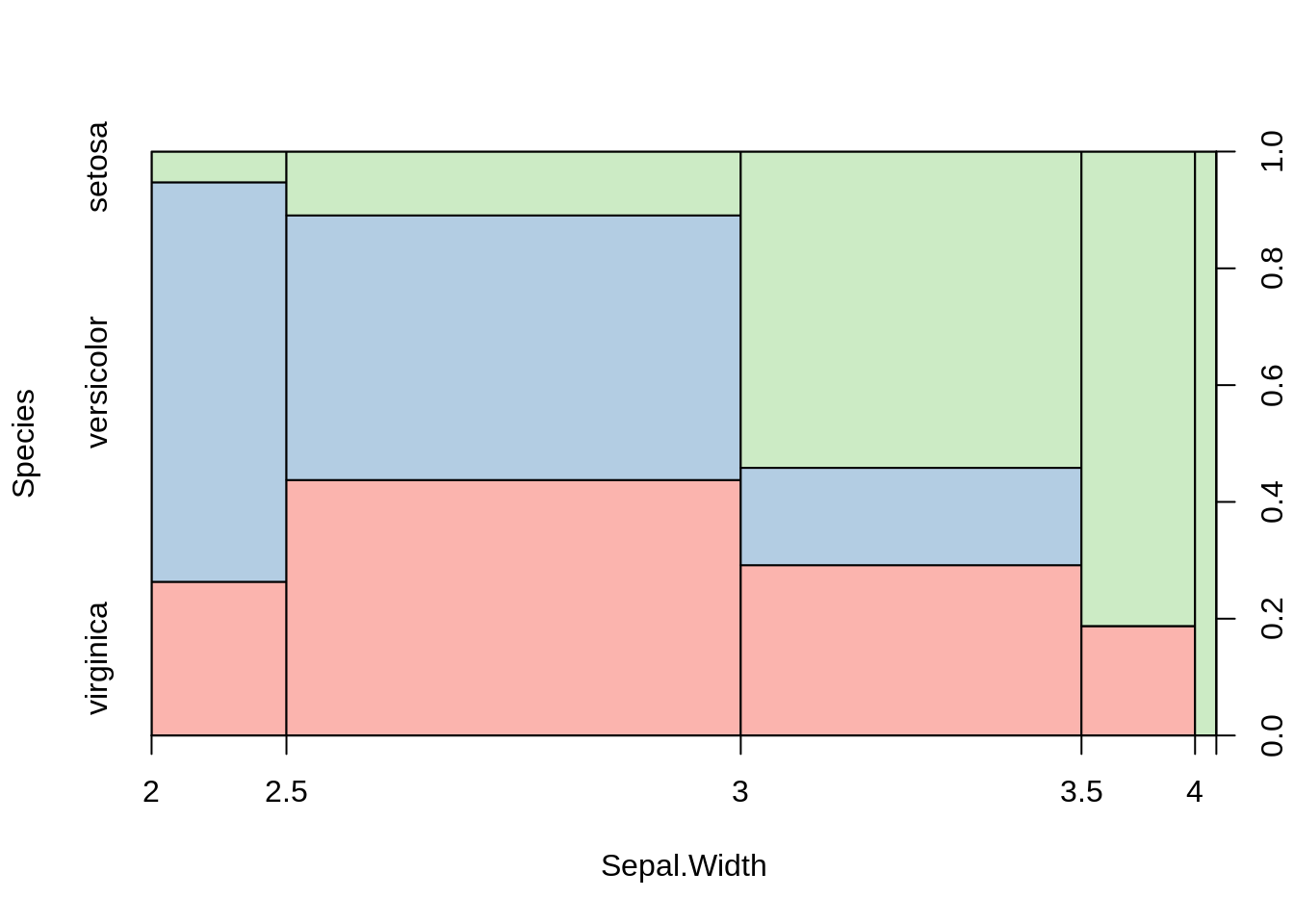
# More idiomatic tinyplot way of drawing the previous plot: use y == by
tinyplot(
  Species ~ Sepal.Width | Species, data = iris,
  type = type_spineplot(breaks = 4),
  palette = "Pastel 1", legend = FALSE
)

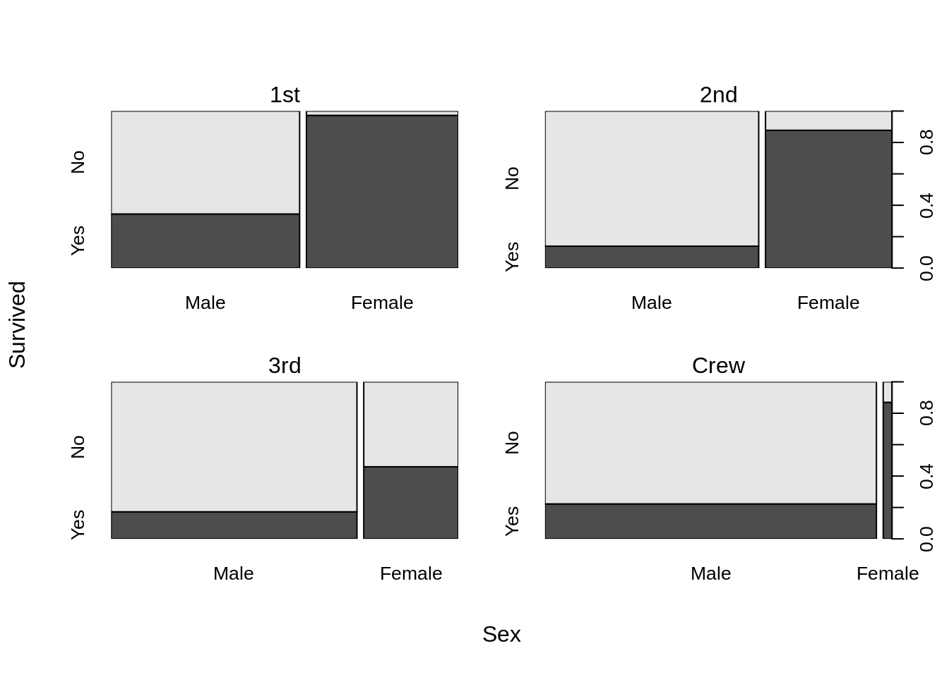
## Grouped and faceted spineplots

ttnc = as.data.frame(Titanic)

# Note: The Titanic (ttnc) dataset is pre-tabulated, so we pass its frequency
# counts via the top-level `weights` argument (accepted via non-standard
# evaluation in the formula method).
tinyplot(
  Survived ~ Sex, facet = ~ Class, data = ttnc,
  # type_spineplot(weights = ttnc$Freq), ## same thing but not NSE
  type = "spineplot", weights = Freq
)

# Reorder x and y variable categories either by their character levels or
# numeric indexes. (Here we combine a top-level `weights` with constructor-
# level arguments passed through `type_spineplot()`.)
tinyplot(
  Survived ~ Sex, facet = ~ Class, data = ttnc,
  type = type_spineplot(xlevels = c("Female", "Male"), ylevels = 2:1),
  weights = Freq
)

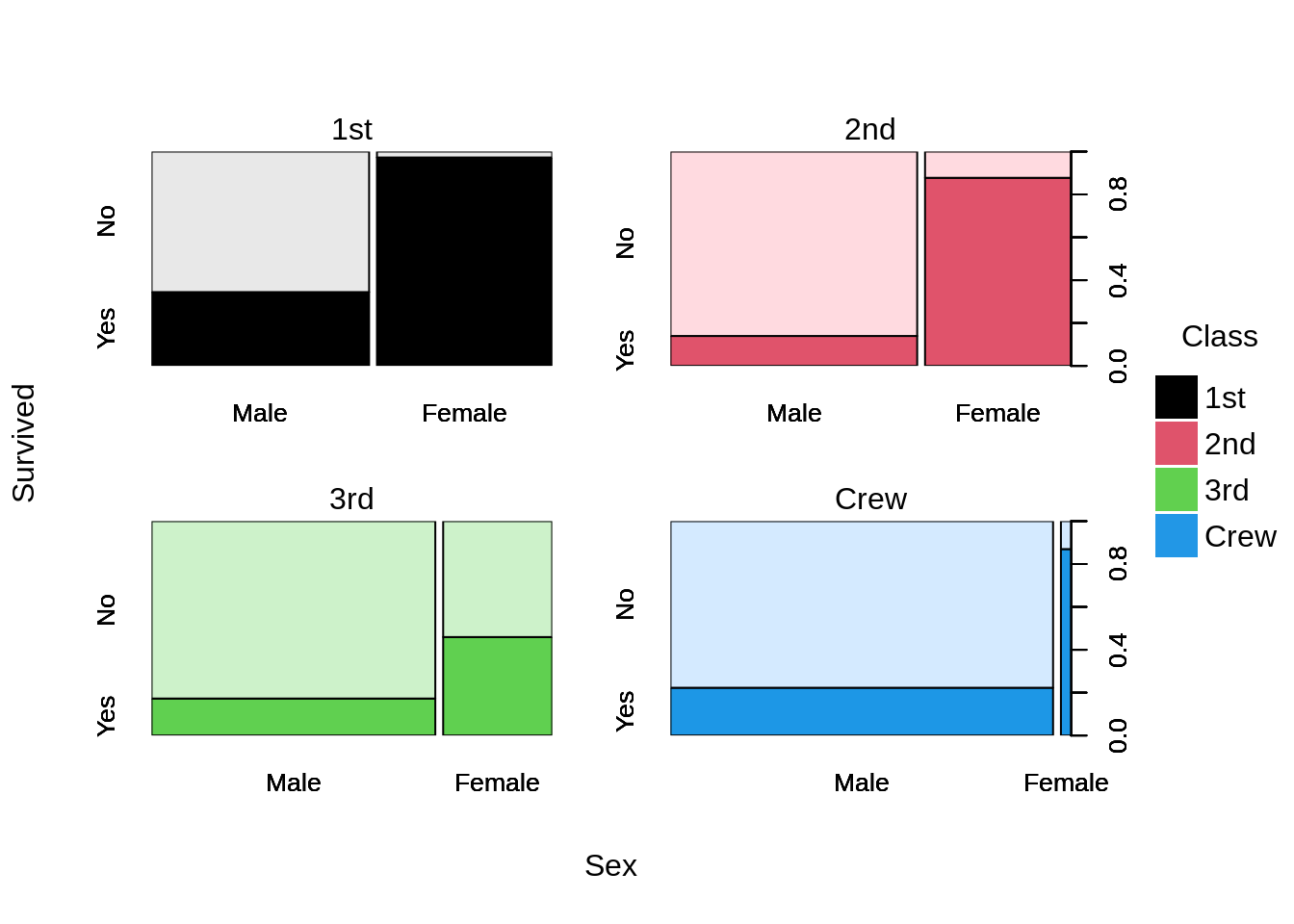
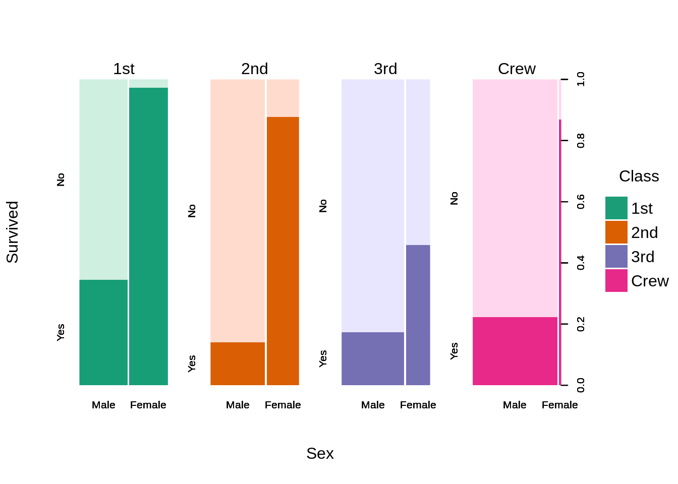
# For (colour) grouped "by" spineplots, it's visually better to facet too
tinyplot(
  Survived ~ Sex | Class, data = ttnc,
  facet = "by",
  type = "spineplot", weights = Freq
)

# Fancier version. Note the smart inheritance of spacing etc.
tinyplot(
  Survived ~ Sex | Class, data = ttnc,
  facet = "by", facet.args = list(nrow = 1),
  type = "spineplot", weights = Freq,
  theme = "void", axes = "t", lty = 0, legend = FALSE,
  main = "Who survived the Titanic disaster?",
  sub = "Frequencies by boarding class and sex"
)

# Aside: It's possible to use "by" on its own (without faceting), but the
# overlaid result isn't great. We will likely overhaul this behaviour in a
# future version of tinyplot...
tinyplot(Survived ~ Sex | Class, data = ttnc,
  type = "spineplot", weights = Freq, alpha = 0.3
)