library(tinyplot)

tinytheme("minimal")

tinyplot(
  Sepal.Length ~ Petal.Length | Species,
  data = iris,
  main = "Title of the plot",
  sub = "A smaller subtitle",
  cap = "Source: A helpful caption"
)
The base R aesthetic tends to divide option. Some people like the default minimalist look of base R plots and are happy to customize the (many) graphical parameters that are available to them. Others find base plots ugly and don’t want to spend time endlessly tweaking different parameters. Meanwhile, the “canvas” drawing system of base R graphics creates its own set of issues. Each plot element is drawn according to a fixed placement logic, which means that the overall composition can’t adjust dynamically according to the elements that are present or not (including titles). This can lead to awkward whitespace artifacts unless the user explicitly accounts for them.
Regardless of where you stand in this debate, the tinyplot view is that base R graphics should ideally combine flexibility and ease of use with aesthetically pleasing end results. One way that we enable this is via themes.
tinytheme()The tinytheme() function provides a mechansim for easily changing the look of your plots to match a variety of pre-defined styles. Behind the scenes, this works by simultaneously setting a group of graphical parameters to achieve a particular aesthetic. Let’s take a look at the “minimal” theme for example, which is inspired by a well-known ggplot2 theme.
library(tinyplot)
tinytheme("minimal")
tinyplot(
Sepal.Length ~ Petal.Length | Species,
data = iris,
main = "Title of the plot",
sub = "A smaller subtitle",
cap = "Source: A helpful caption"
)
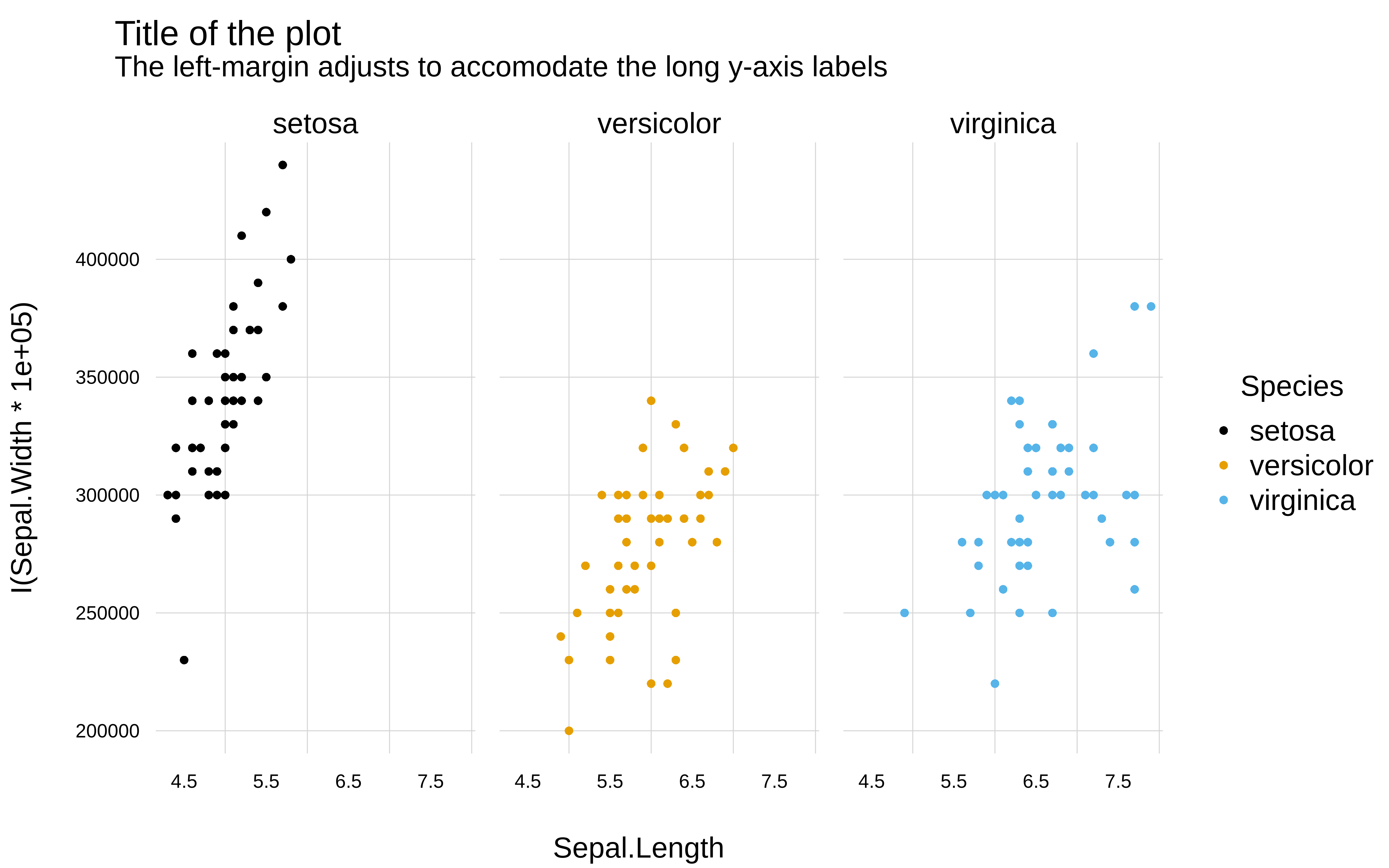
One particular feature that may interest users is the fact that tinytheme() uses some internal magic logic to dynamically adjust plot margins to avoid whitespace and overlapping elements. For example, notice how the plot region here bumps out to accomodate the long horizontal y-axis labels:
tinyplot(
  I(Sepal.Length*1e5) ~ Petal.Length | Species,
  data = iris,
  yaxl = ",",  # use comma format for the y-axis labels
  main = "Title of the plot",
  sub = "A smaller subtitle",
  cap = "Note: The left-margin adjusts to accomodate the long y-axis labels"
)
As you may have noticed, the changes made by tinytheme() are persistent, and apply to all subsequent tinyplot() calls.
tinyplot(mpg ~ hp, data = mtcars, main = "Fuel efficiency vs. horsepower")
To reset graphical parameters to factory defaults, call tinytheme() without arguments.
tinytheme()
tinyplot(mpg ~ hp, data = mtcars, main = "Fuel efficiency vs. horsepower")
Setting a persistent theme for all of your plots is often convenient. But there are also times where you might prefer an ephemeral theme that only applies to a single plot (plus any added layers). You can invoke such an ephemeral theme by calling the tinyplot(..., theme = <theme>) argument directly.
tinyplot(mpg ~ hp, data = mtcars, main = "Ephemeral theme", theme = "clean")
tinyplot(mpg ~ hp, data = mtcars, main = "Back to the default")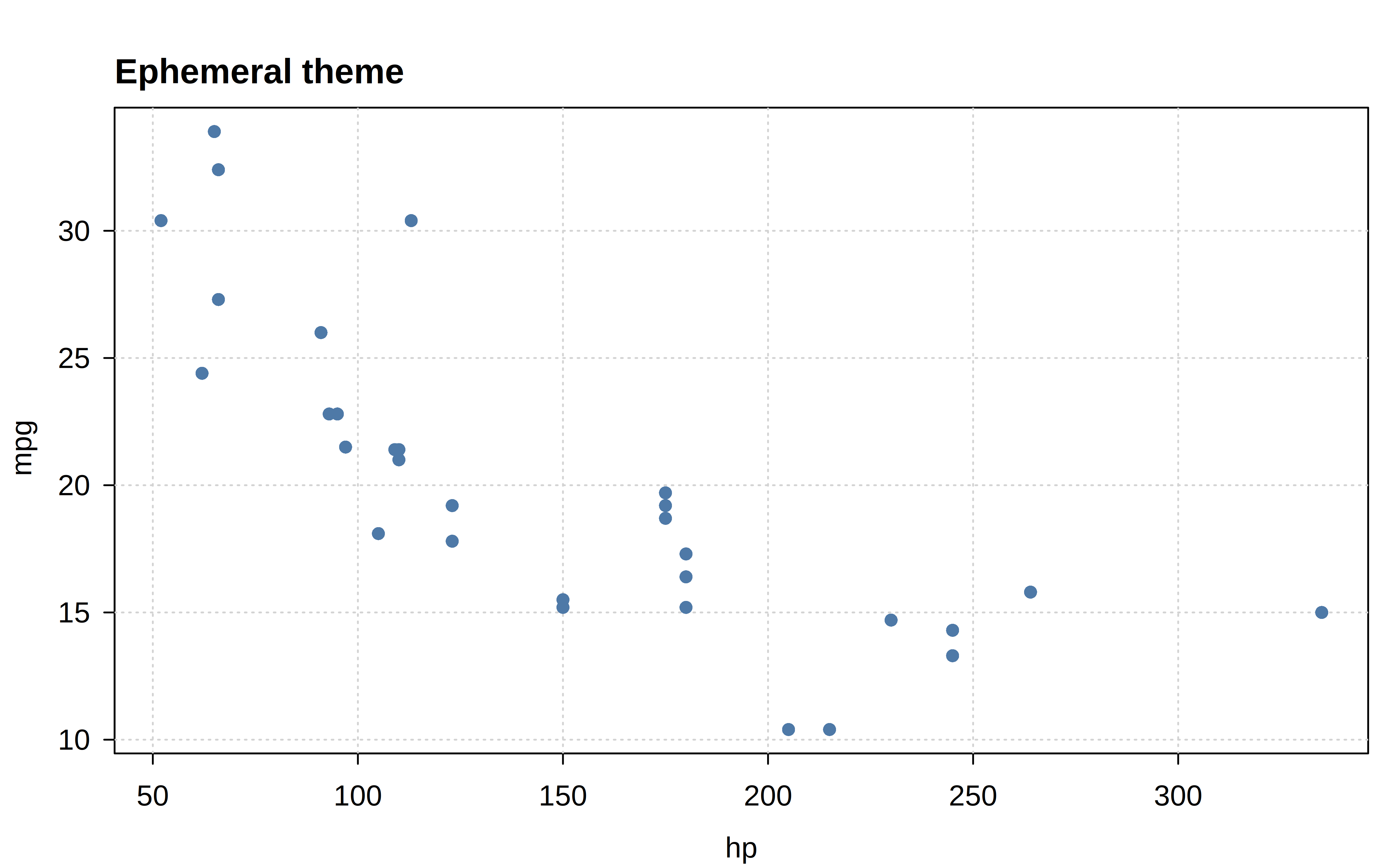
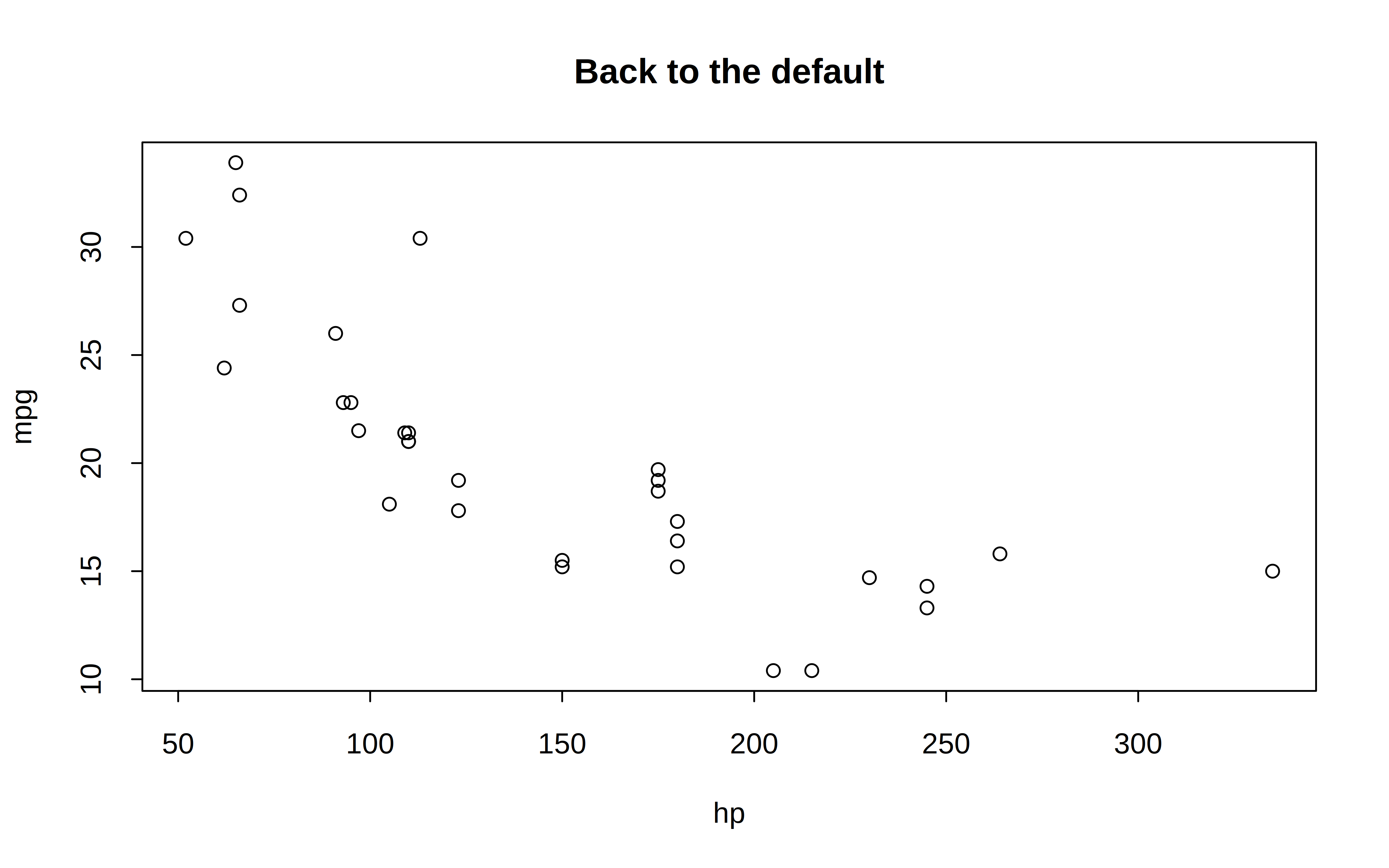
One of the advantages of ephemeral themes is that they won’t interfere with any other base graphics calls (e.g, plot, coplot, etc.) In contrast, the persistent hook mechanism of tinytheme() will also intercept these other base plot calls, which may lead to undesirable outcomes unless you reset to the default behaviour.
We’ll use the following running example to demonstrate the full gallery of built-in tinyplot themes.
p = function(theme = "default") {
  tinyplot(
    bill_len ~ body_mass | species,
    facet = ~sex,
    data = penguins,
    main = paste0('theme = "', theme, '"'),
    sub = "subtitle",
    cap = "caption",
    yaxl = ",",
    theme = theme
  )
  box("outer", lty = 2)
}For non-dynamic themes, the sub and cap arguments are effectively subsitutes, and so will clash for these cases below. But they achieve guaranteed separate placement for dynamic themes.
p() ## same as "default"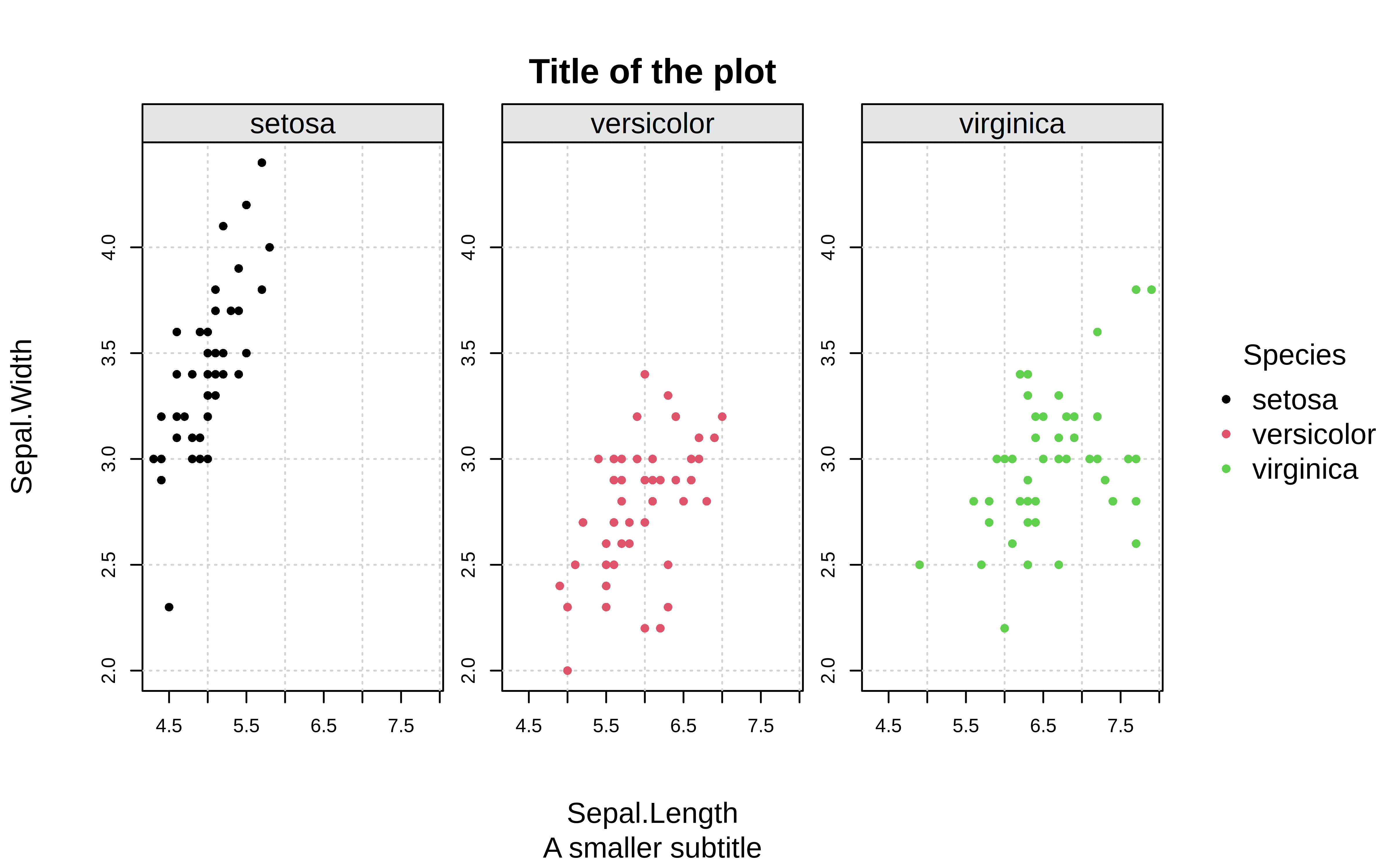
p("basic")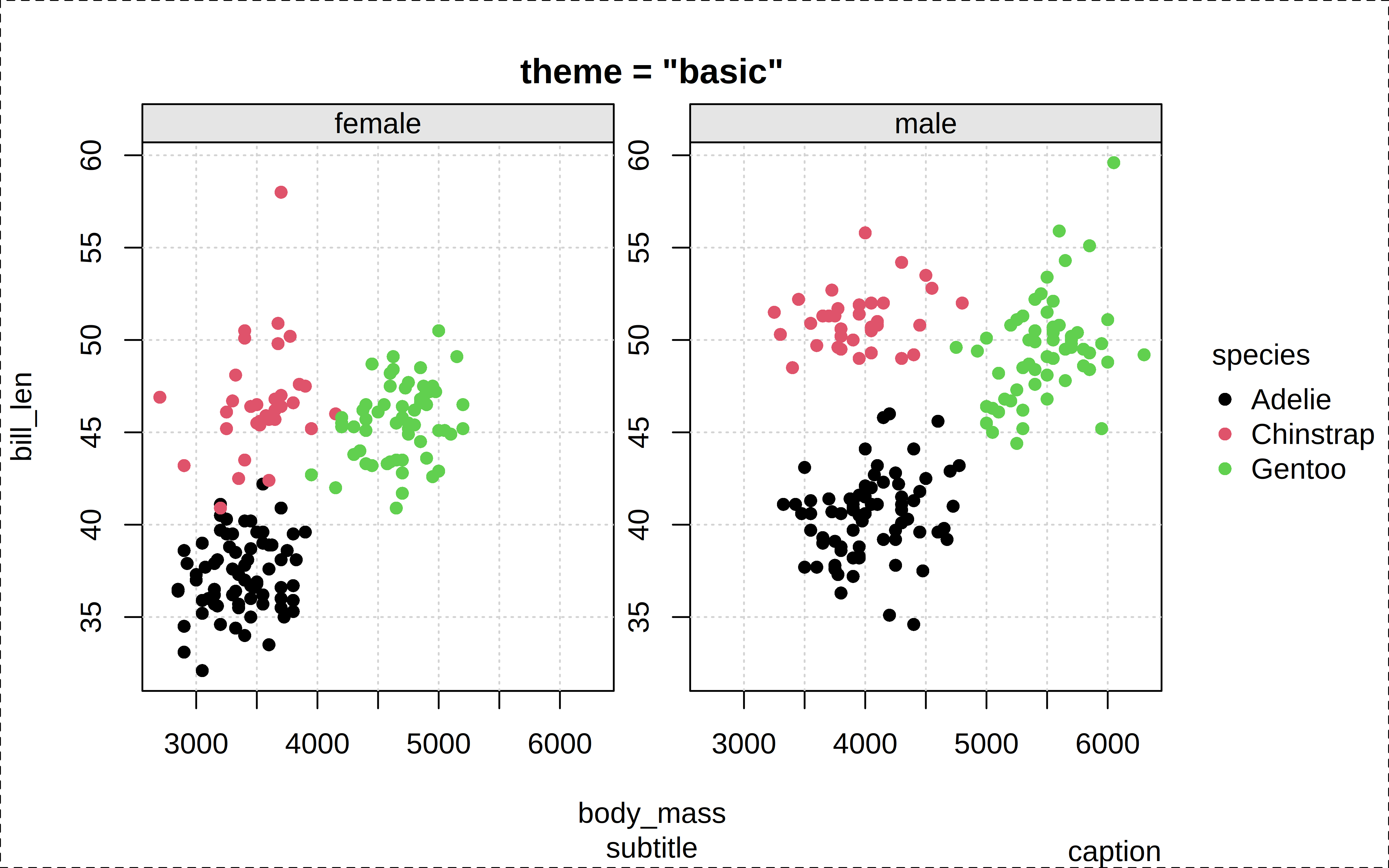
p("dynamic")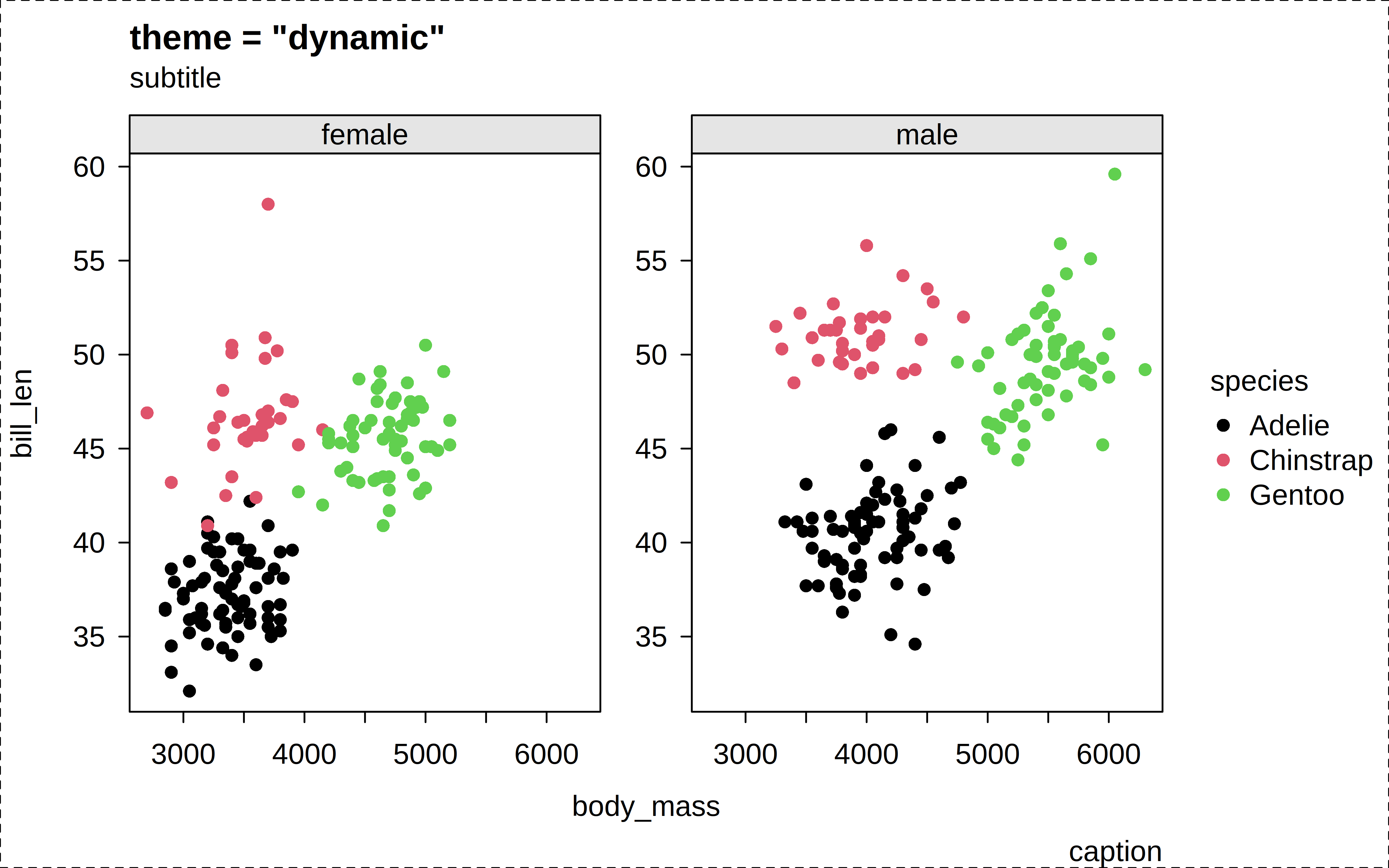
p("clean")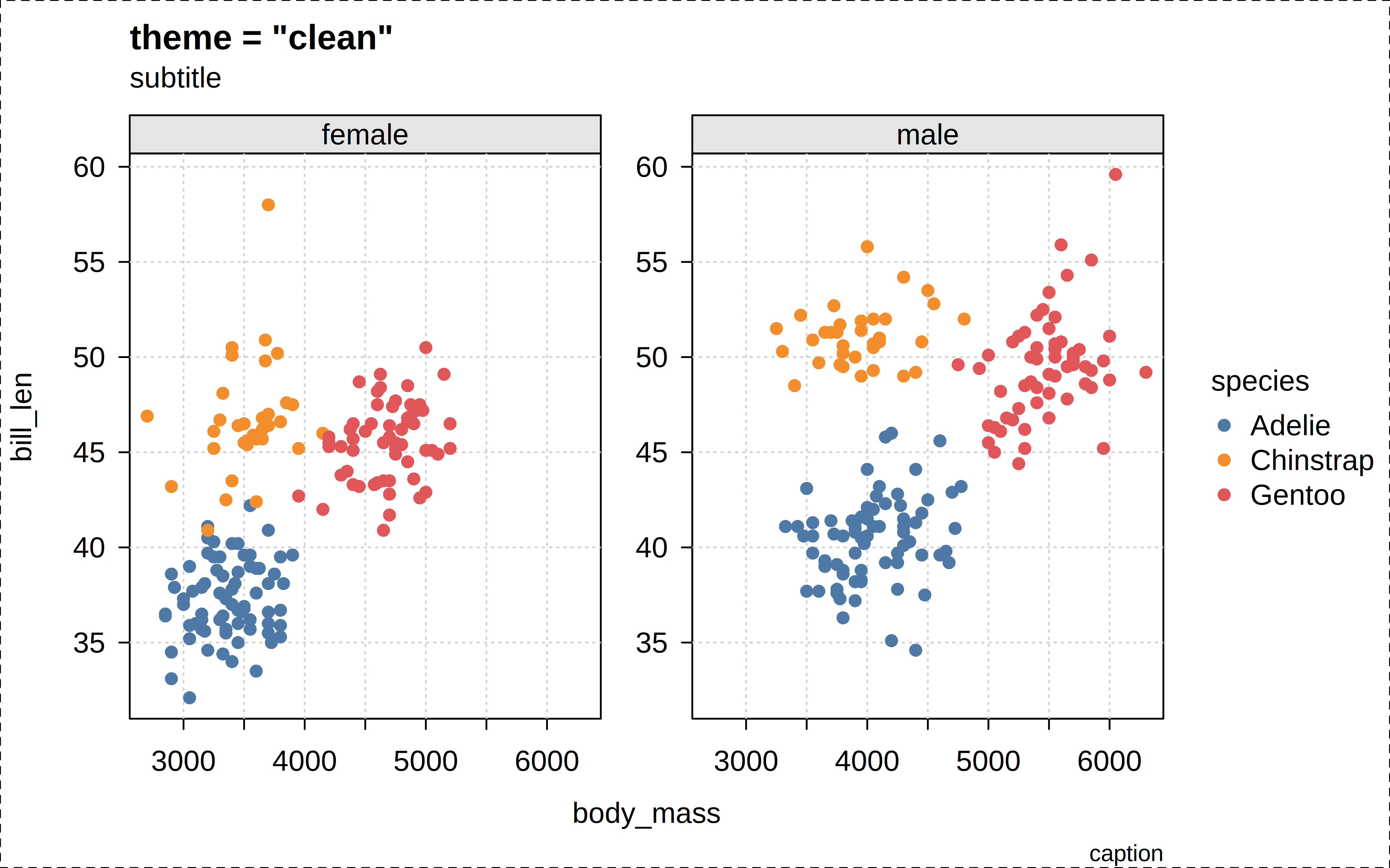
p("clean2")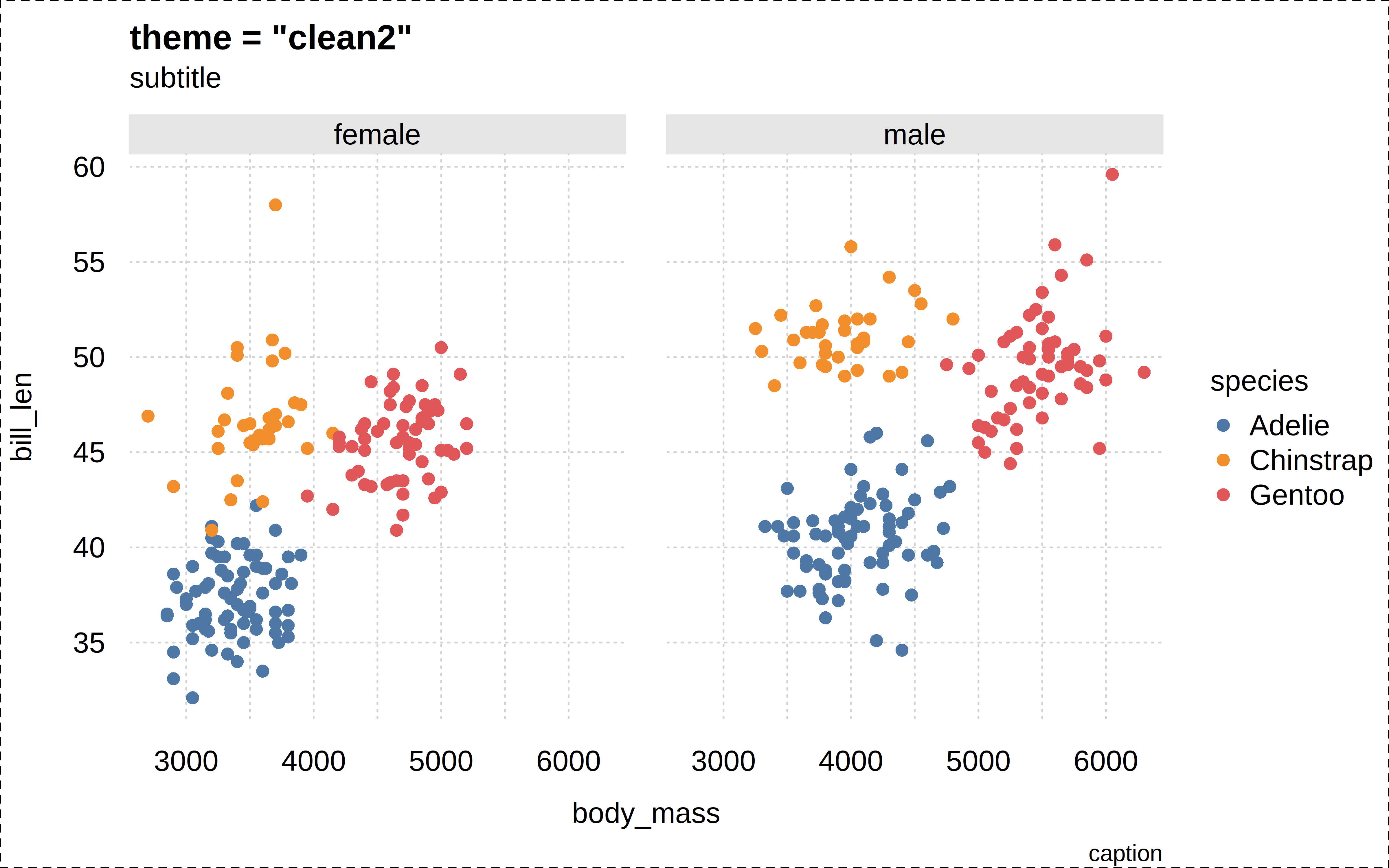
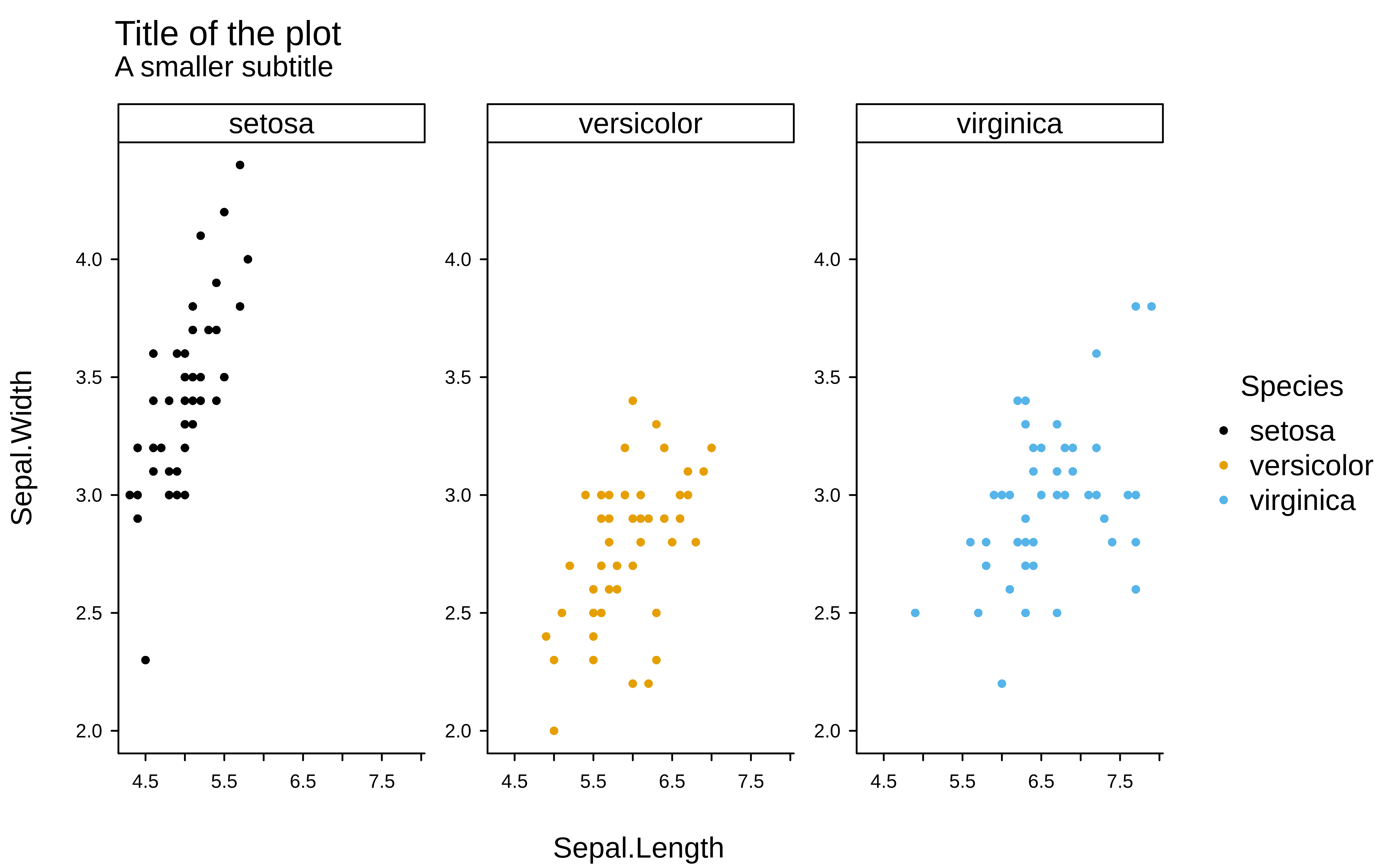
p("classic")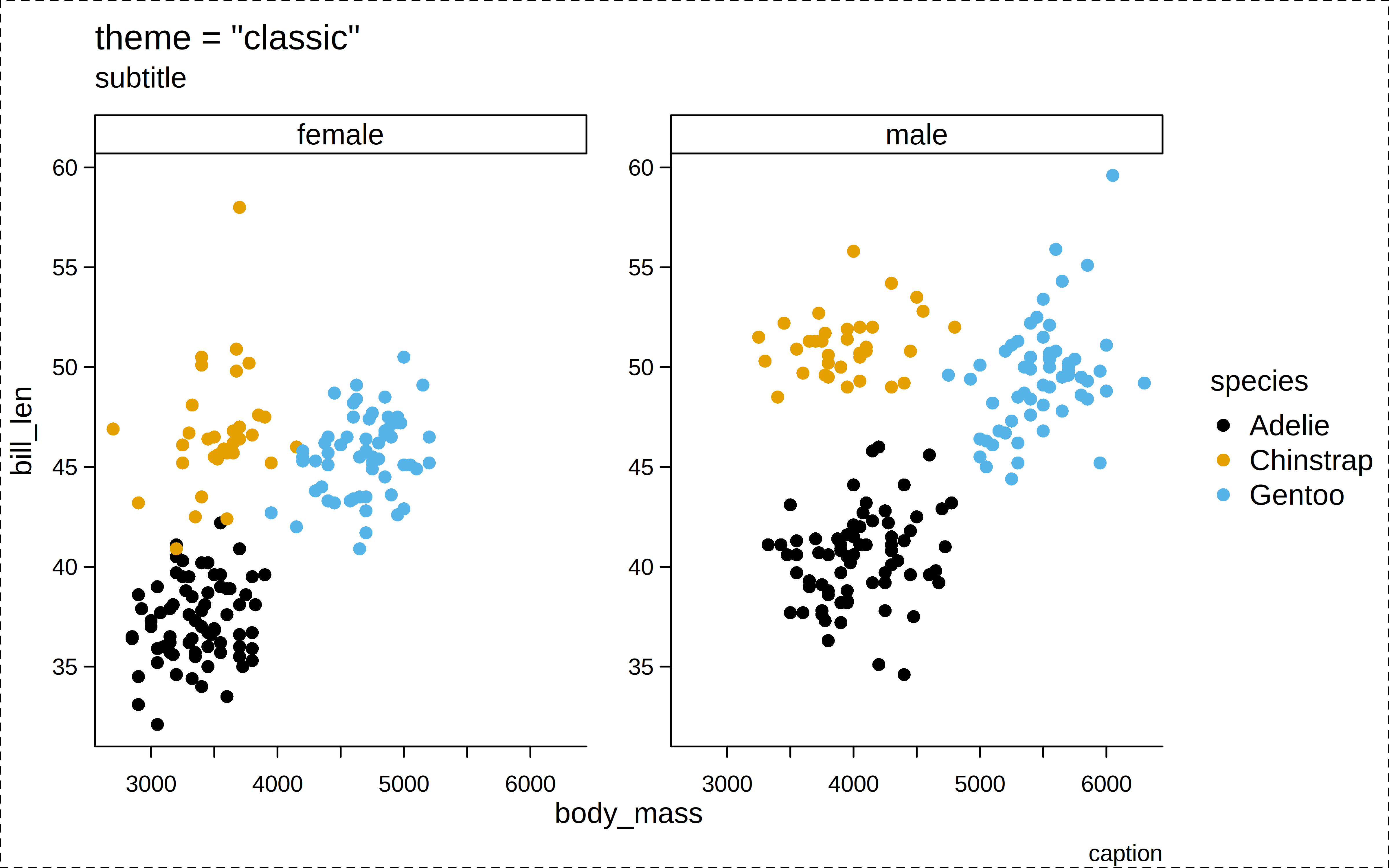
p("bw")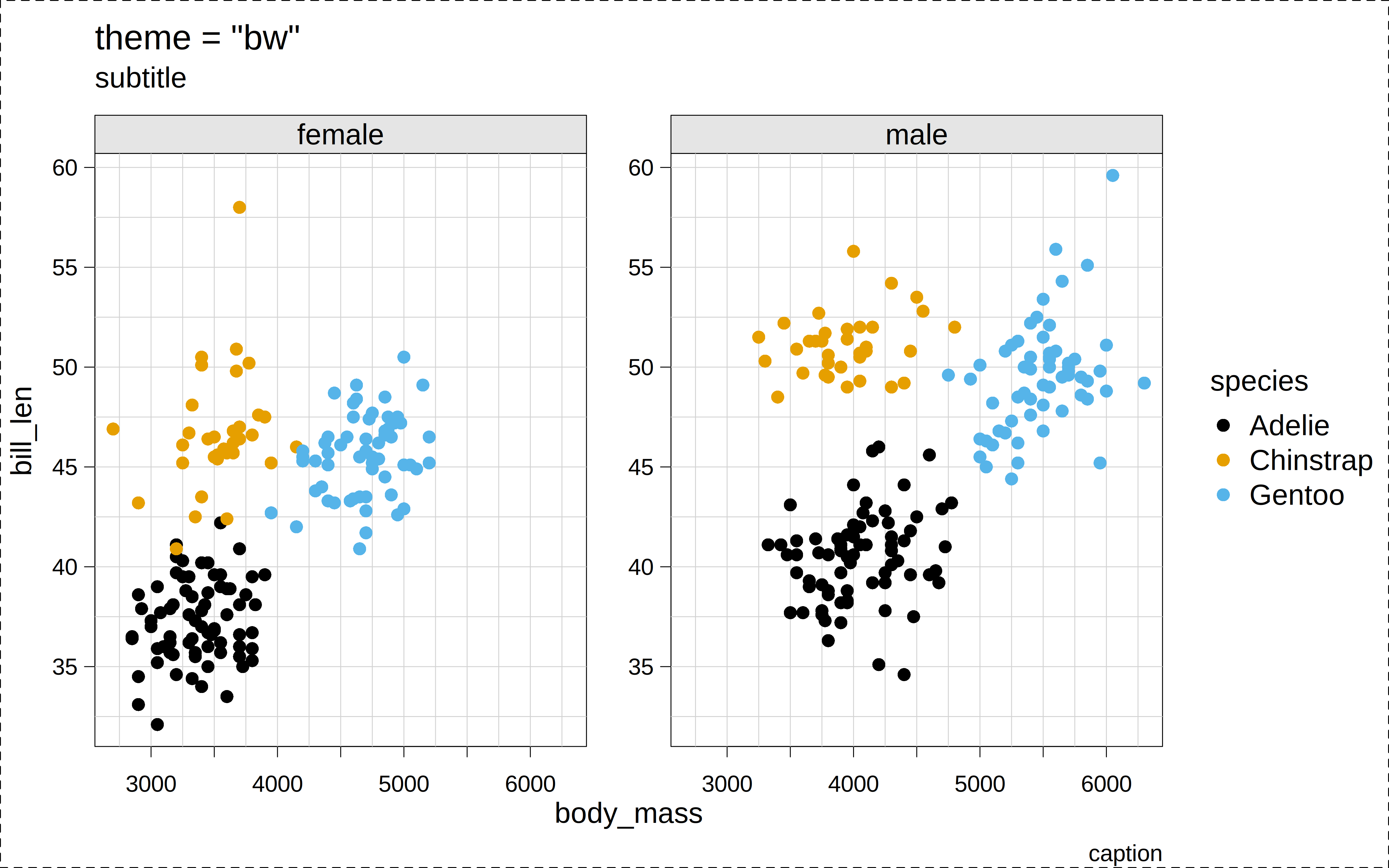
p("linedraw")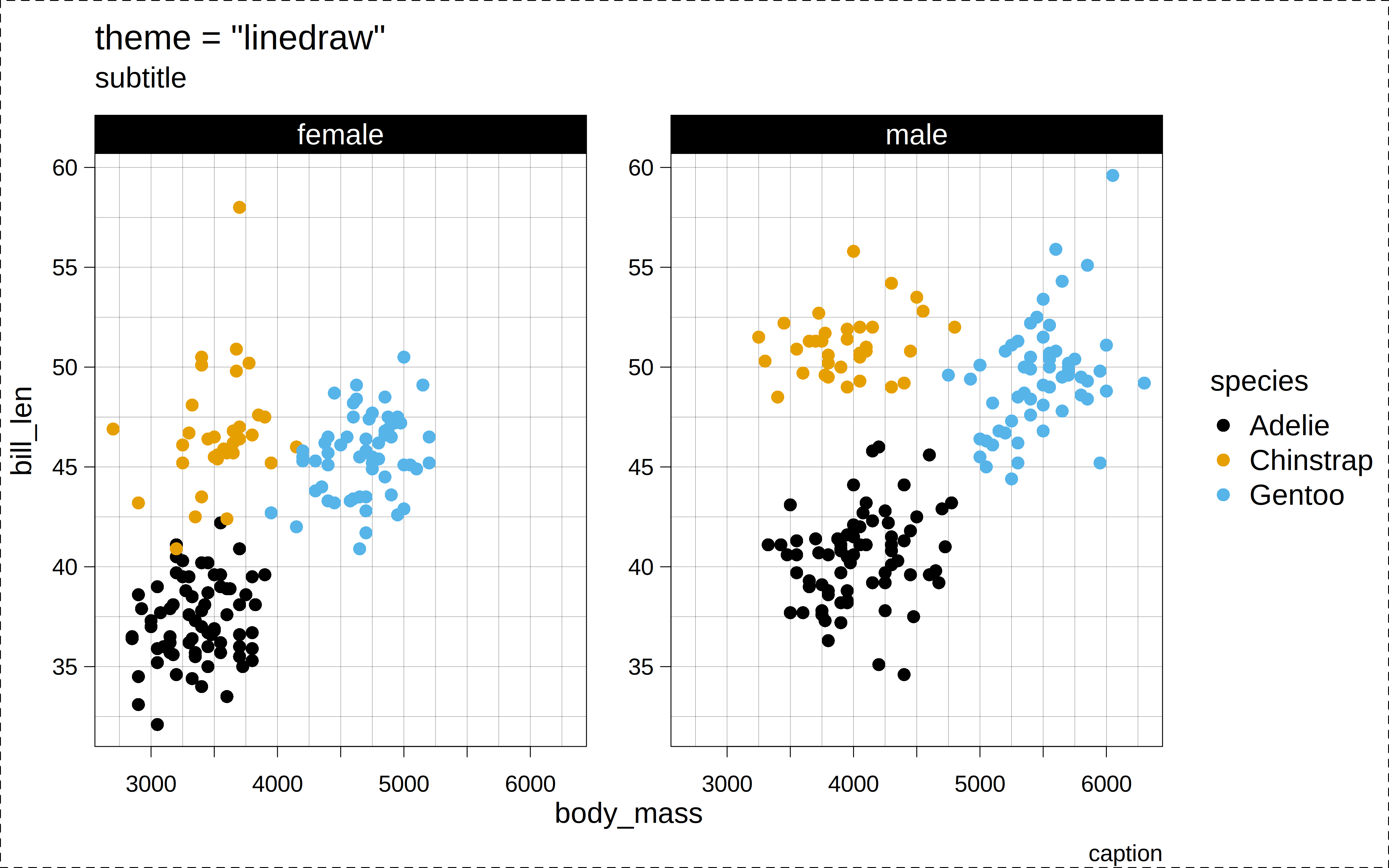
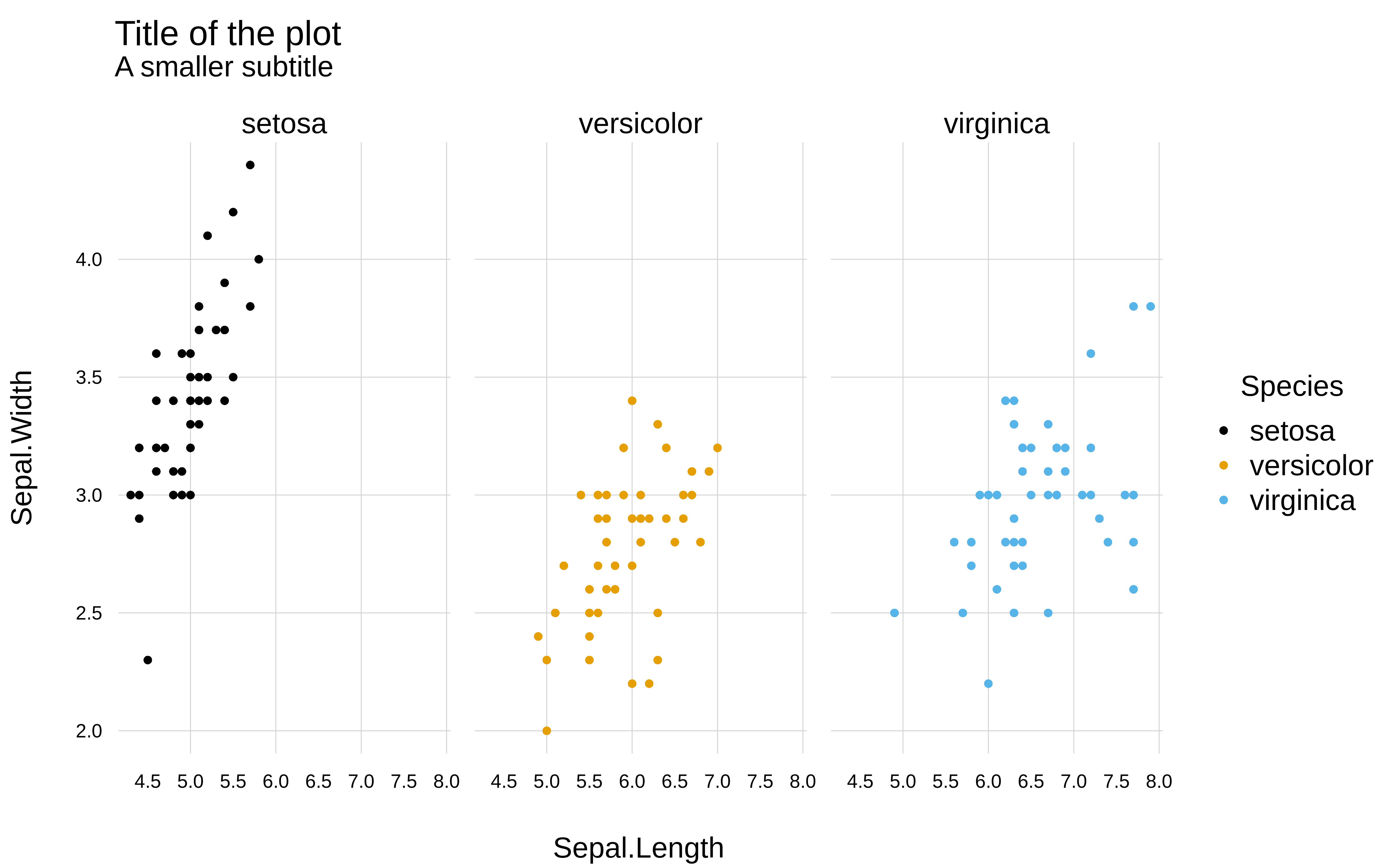
p("minimal")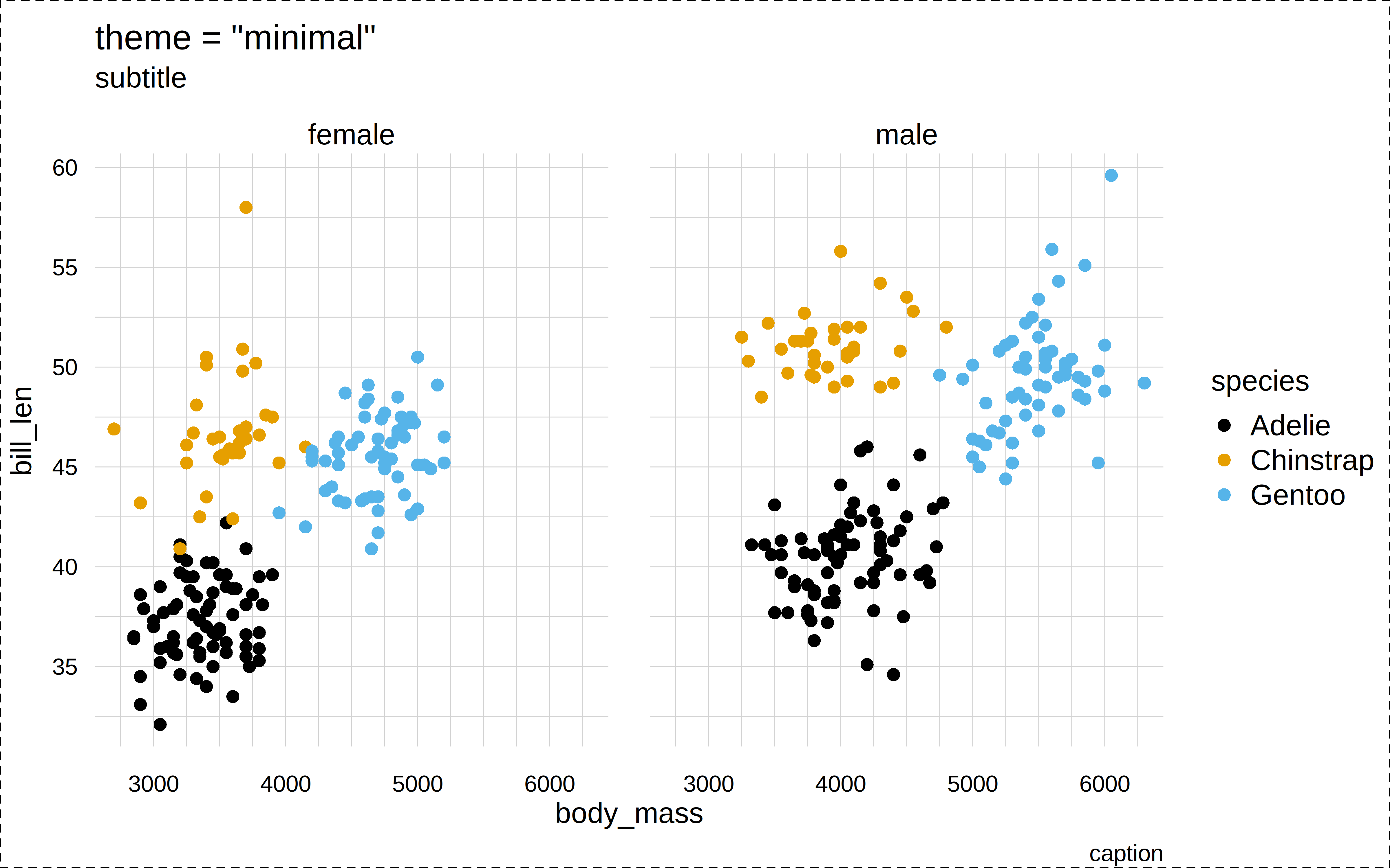
p("ipsum")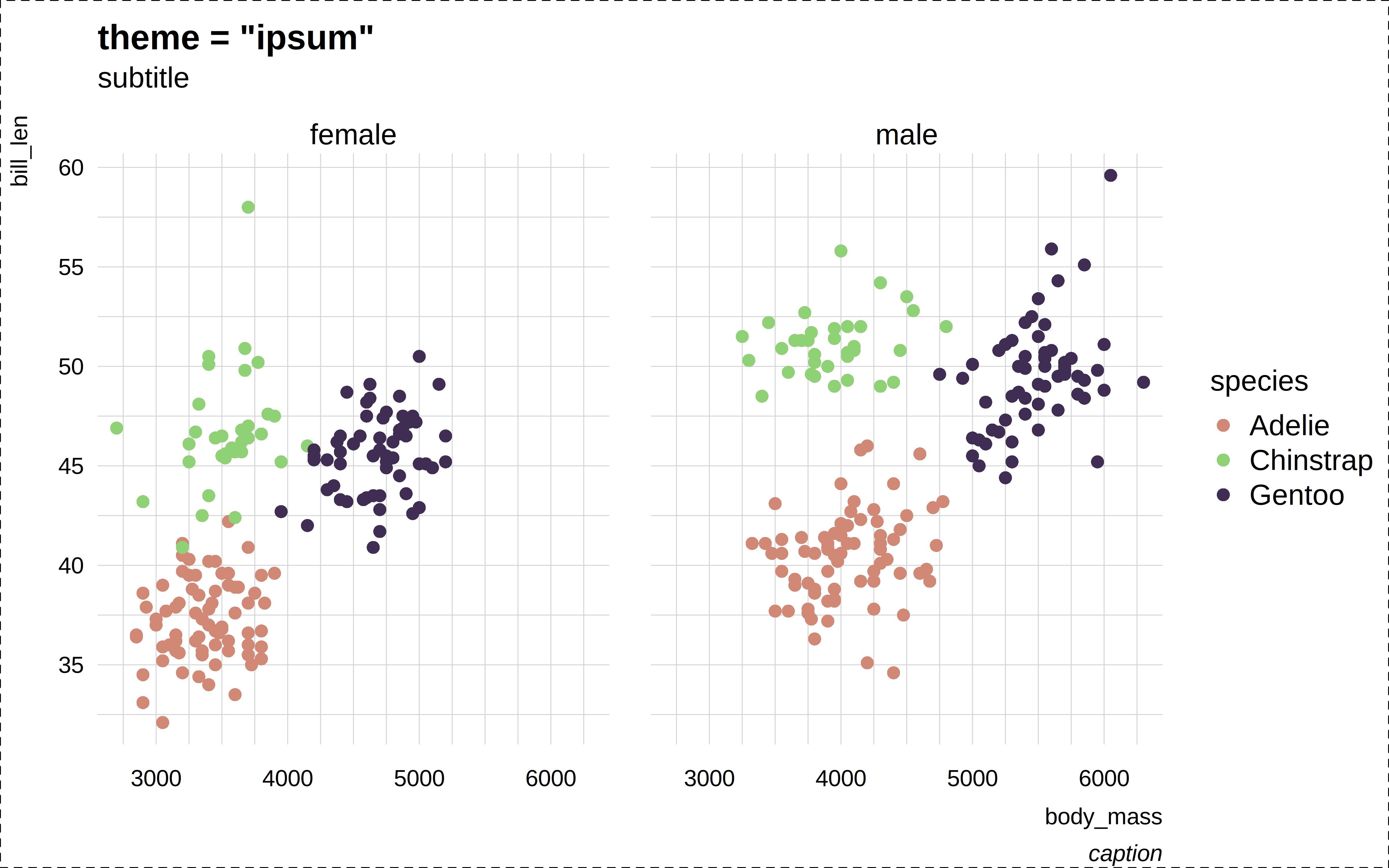
p("ipsum2")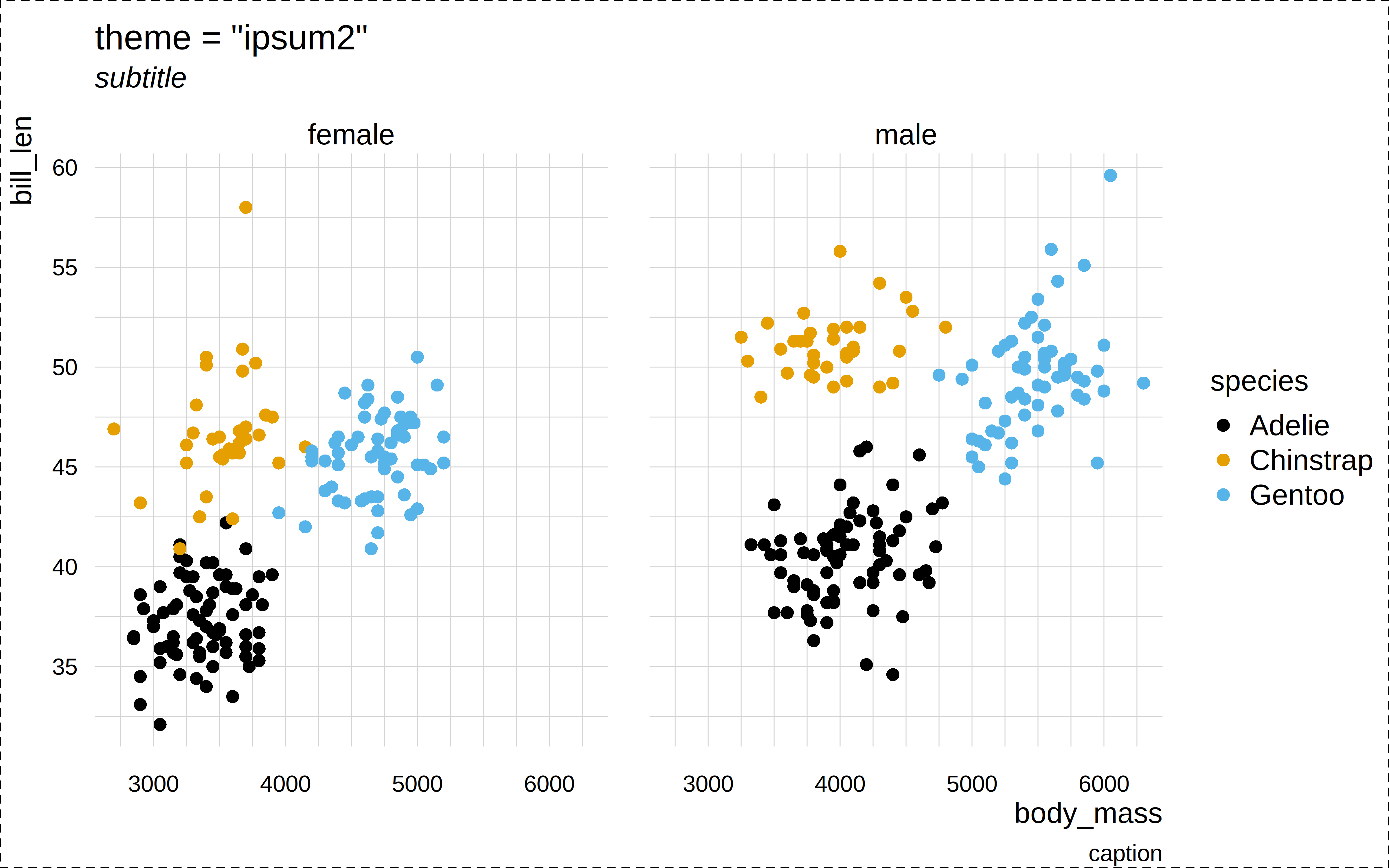
p("dark")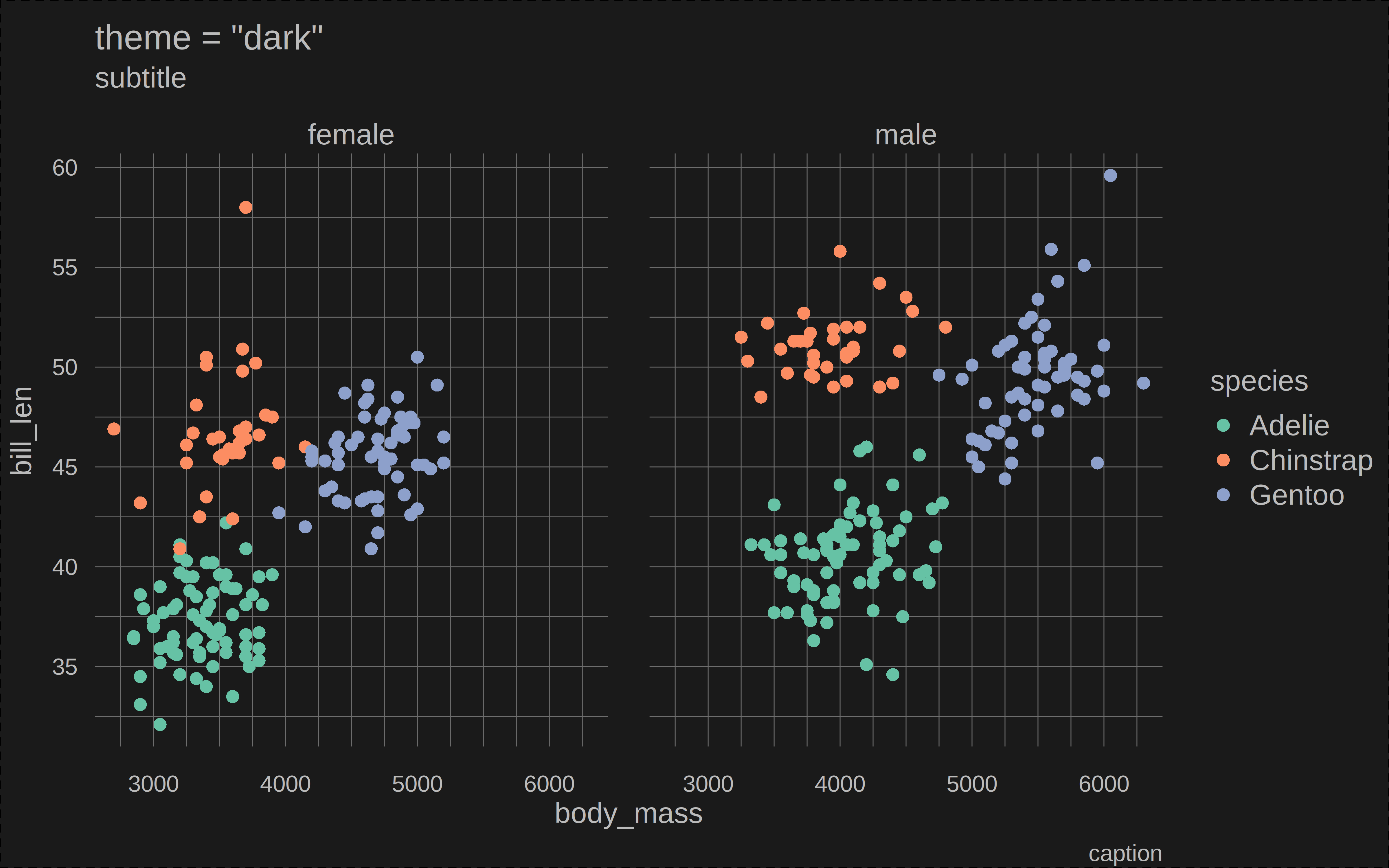
p("socviz")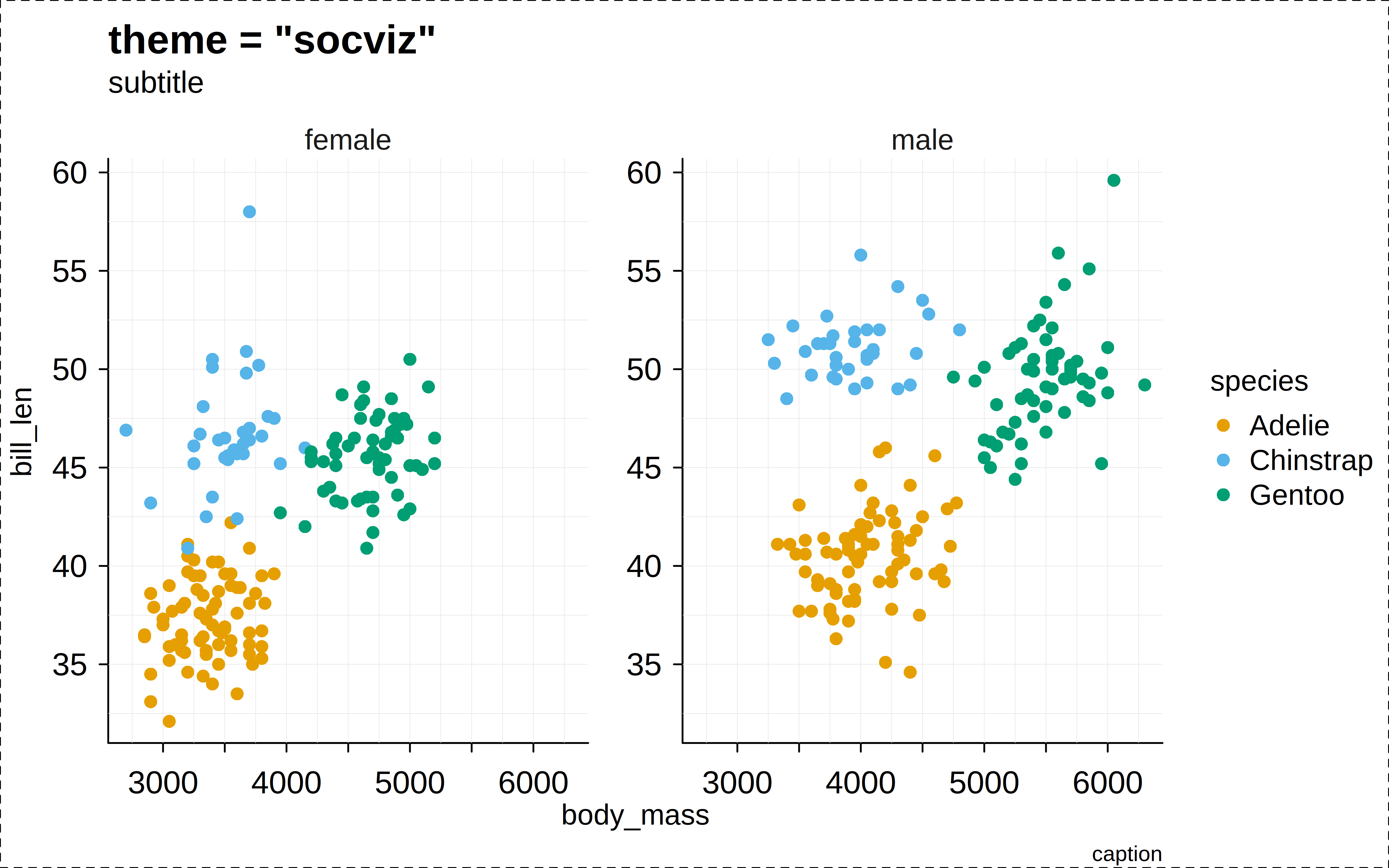
p("broadsheet")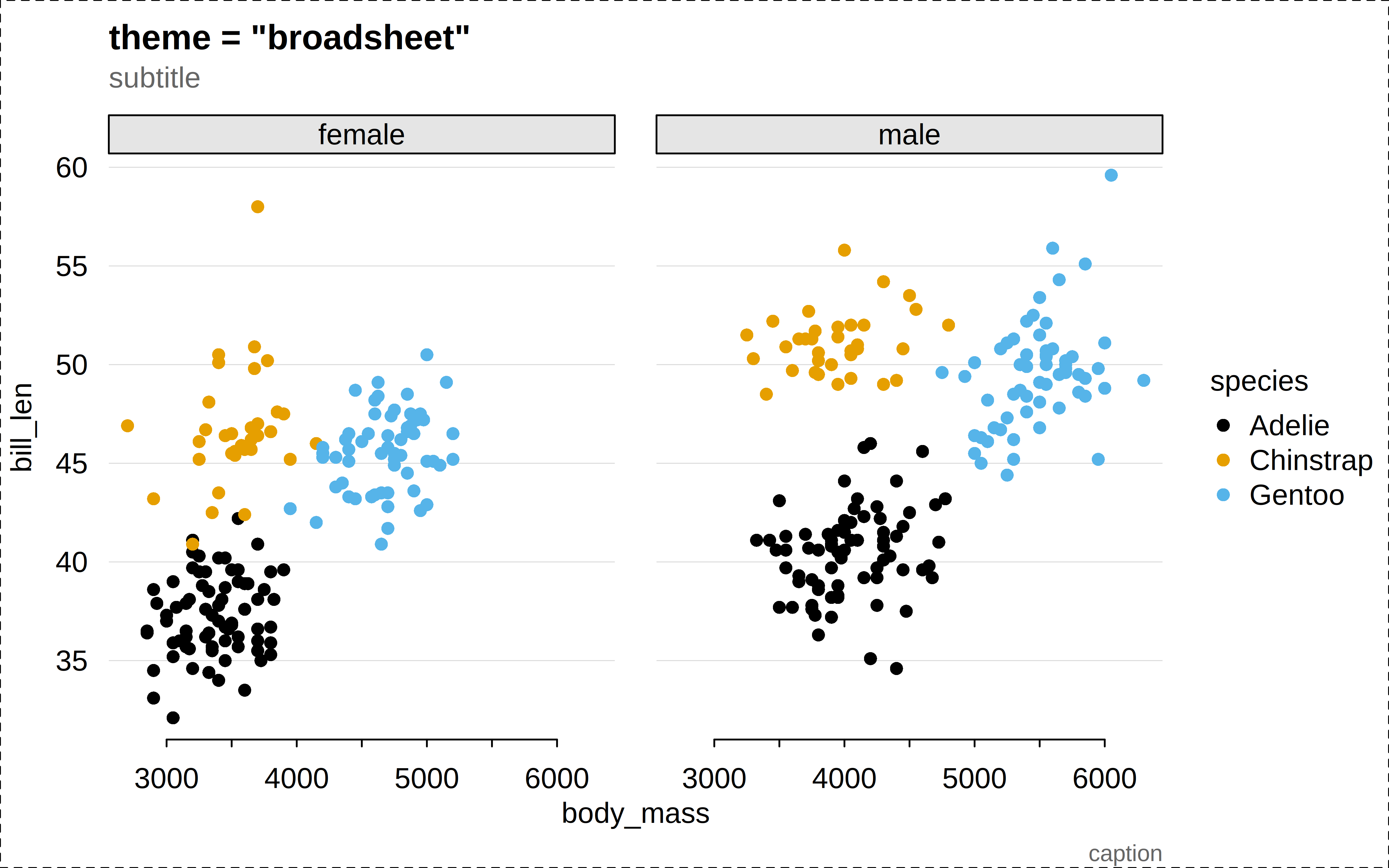
p("nber")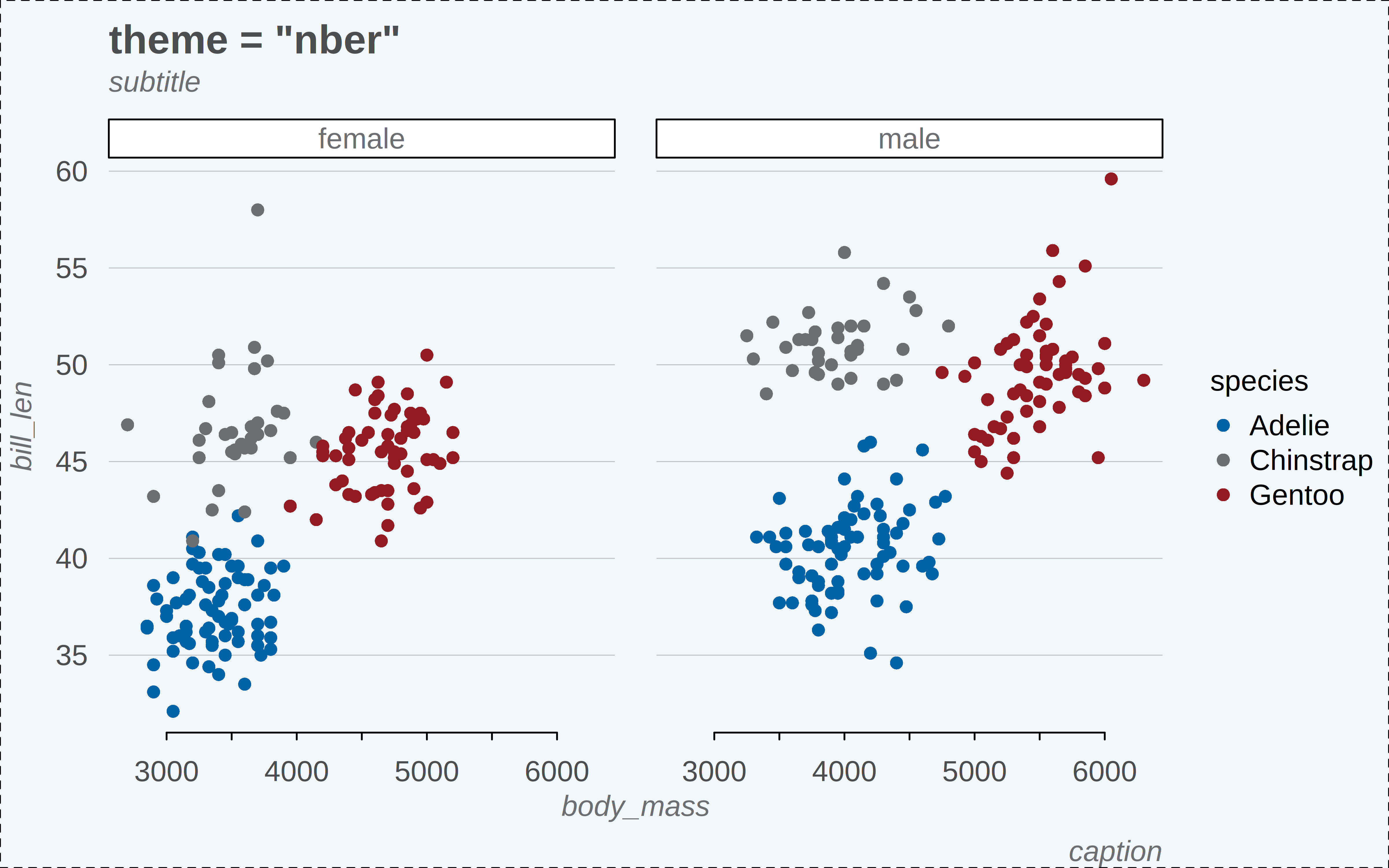
p("web")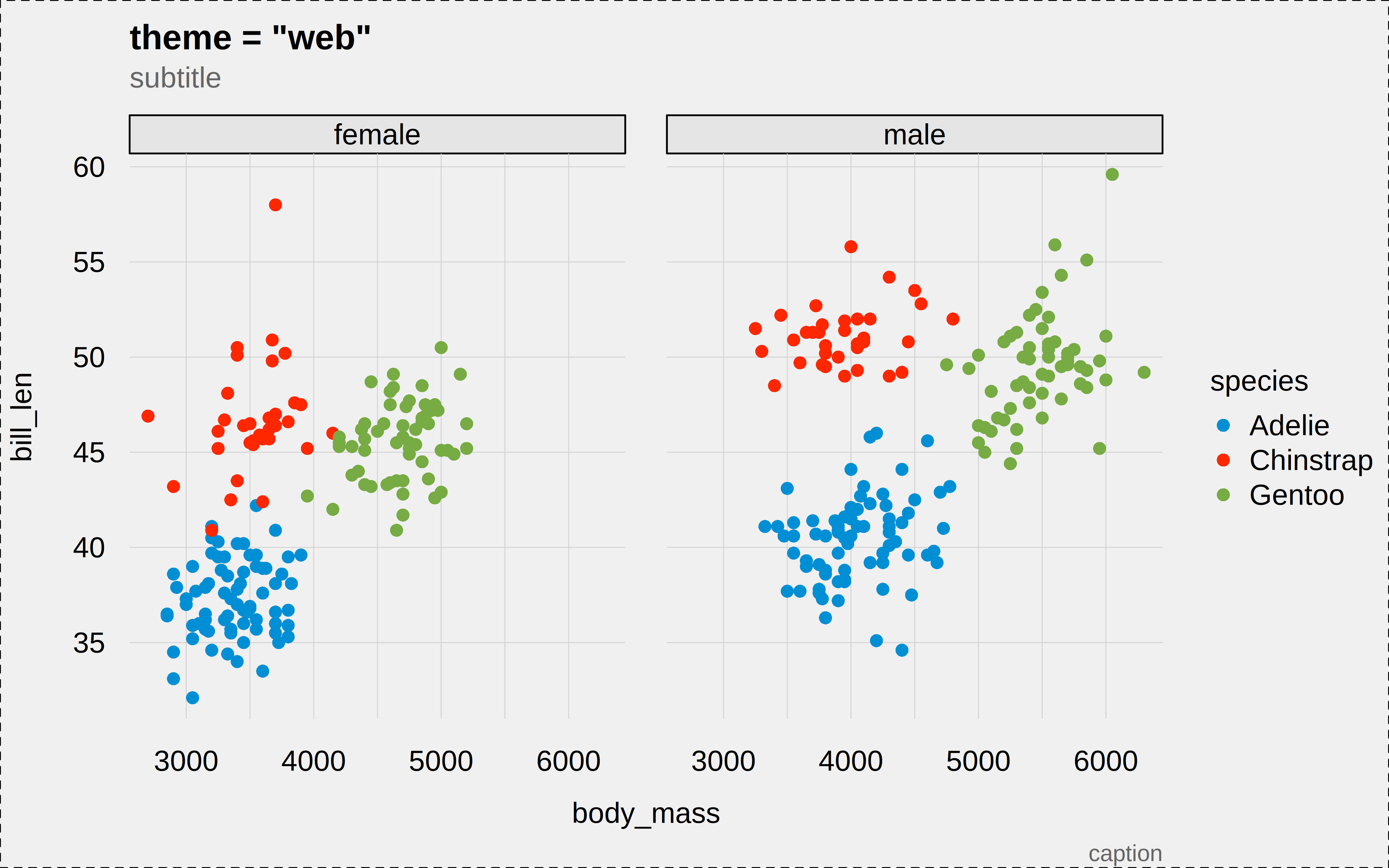
p("tufte")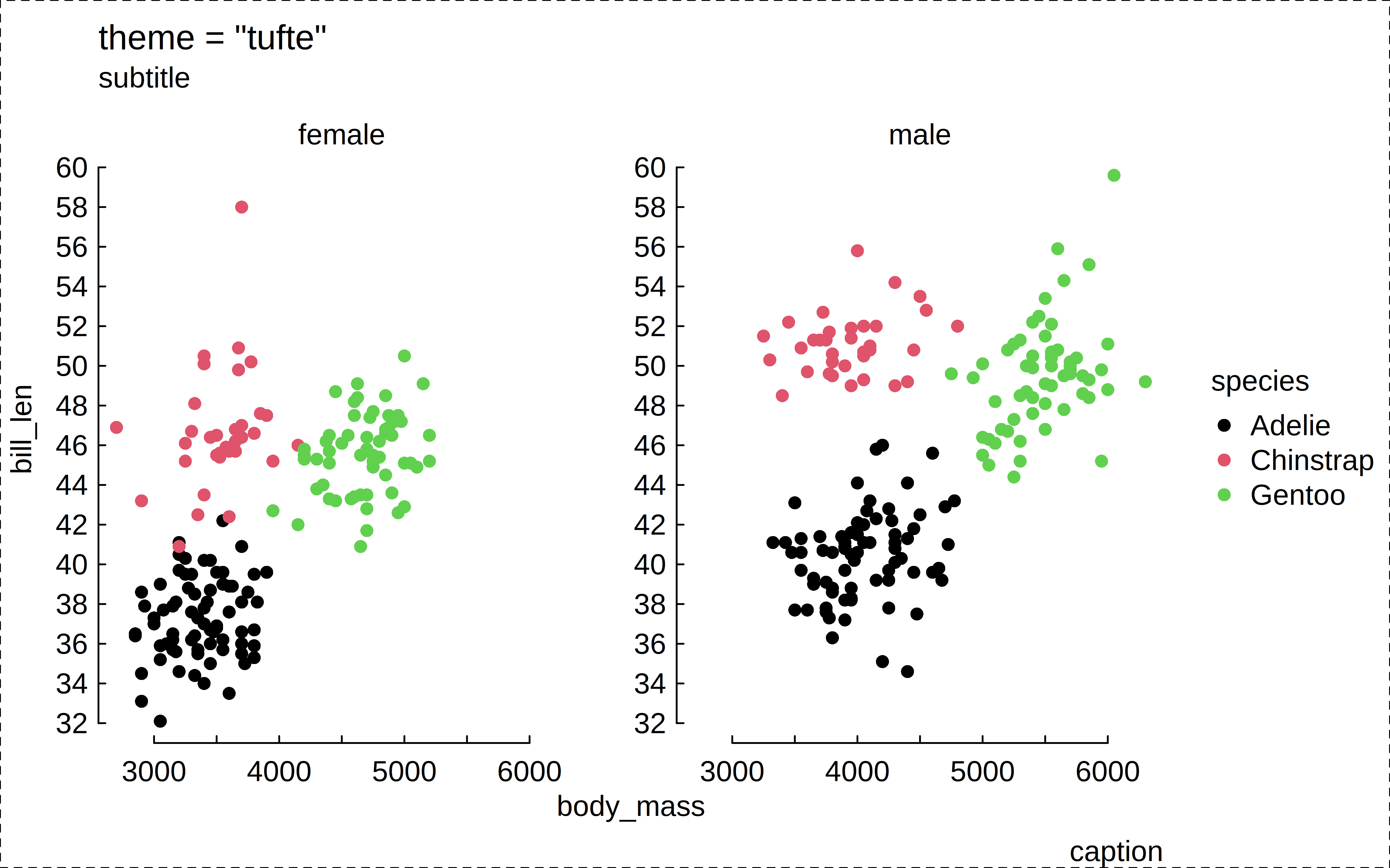
p("float")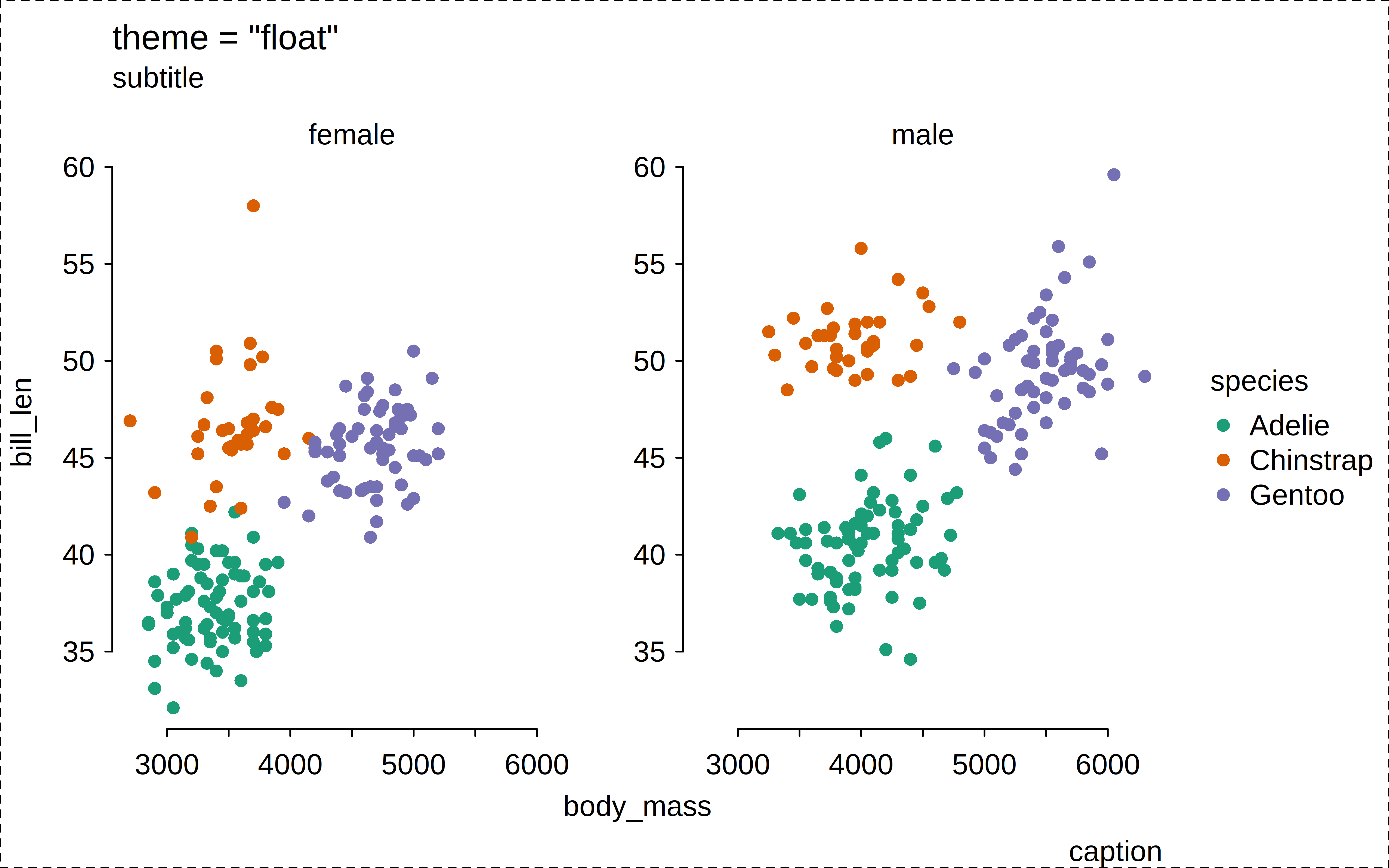
p("void")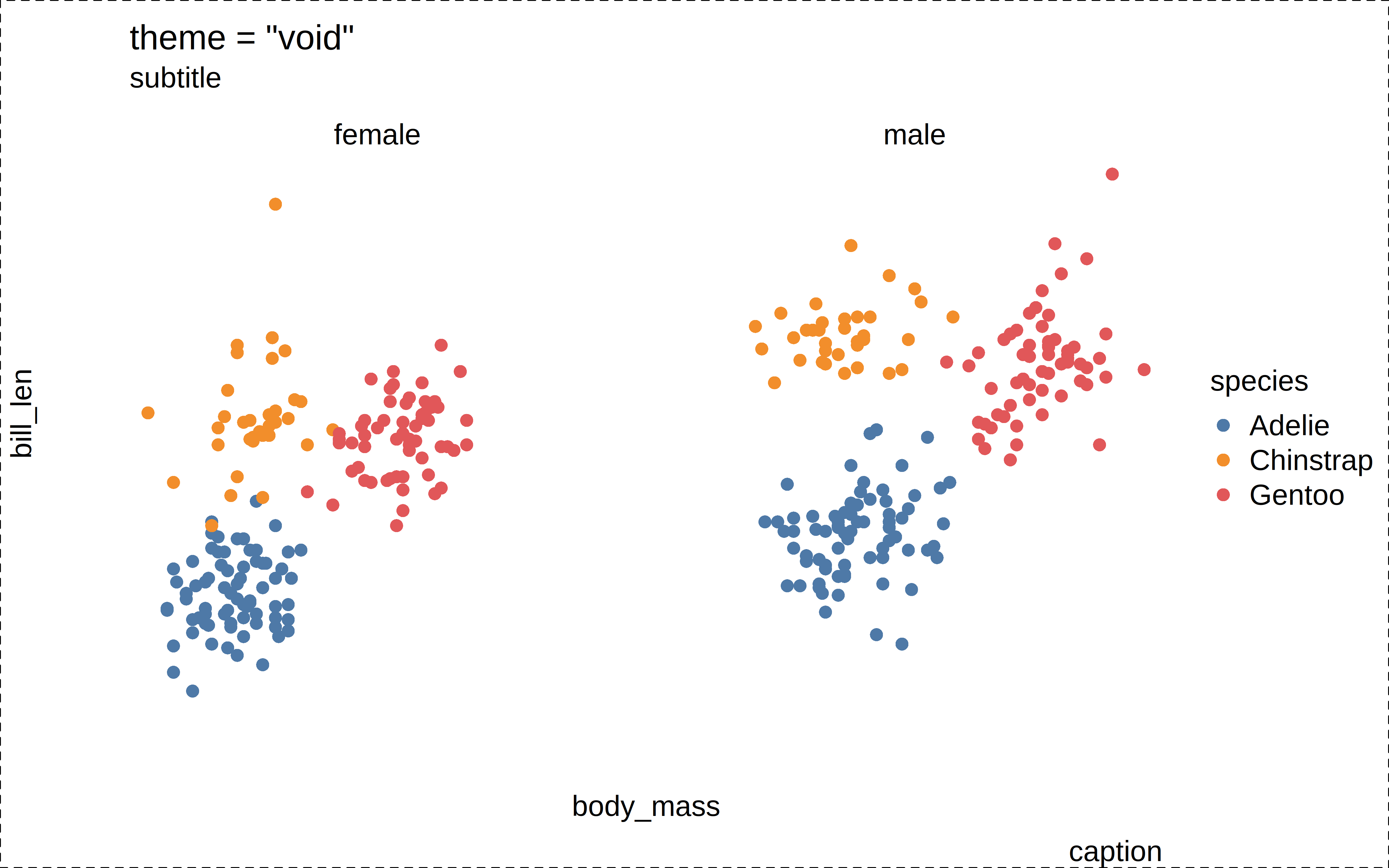
The specialized "ridge" and "ridge2" themes are only intended for use with ridge plot types.
p2 = function(theme = "ridge") {
  tinyplot(
    species ~ body_mass | species,
    data = penguins,
    type = "ridge",
    main = paste0('theme = "', theme, '"'),
    sub = "subtitle",
    cap = "caption",
    theme = theme
  )
  box("outer", lty = 2)
}

p2("ridge")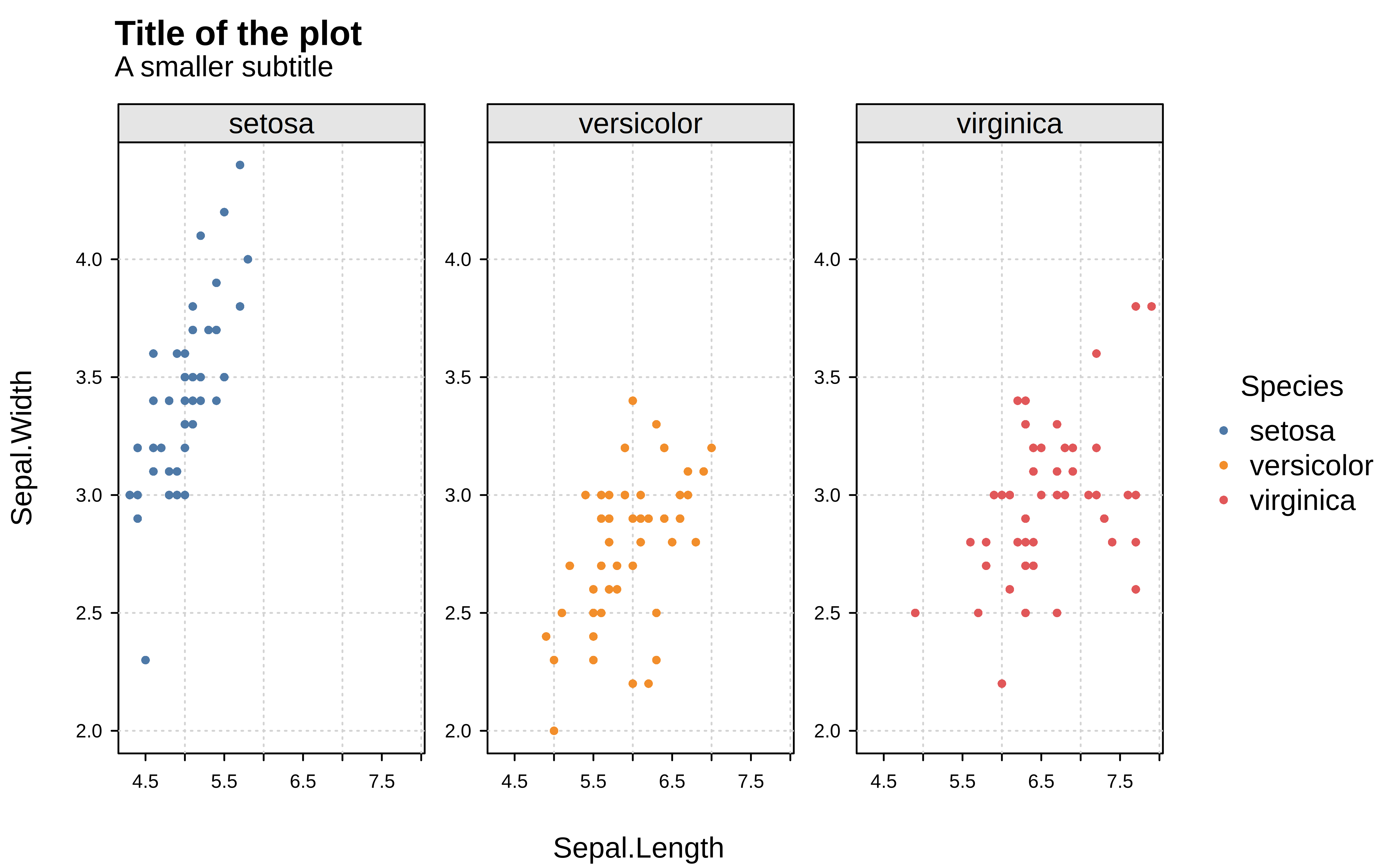
p2("ridge2")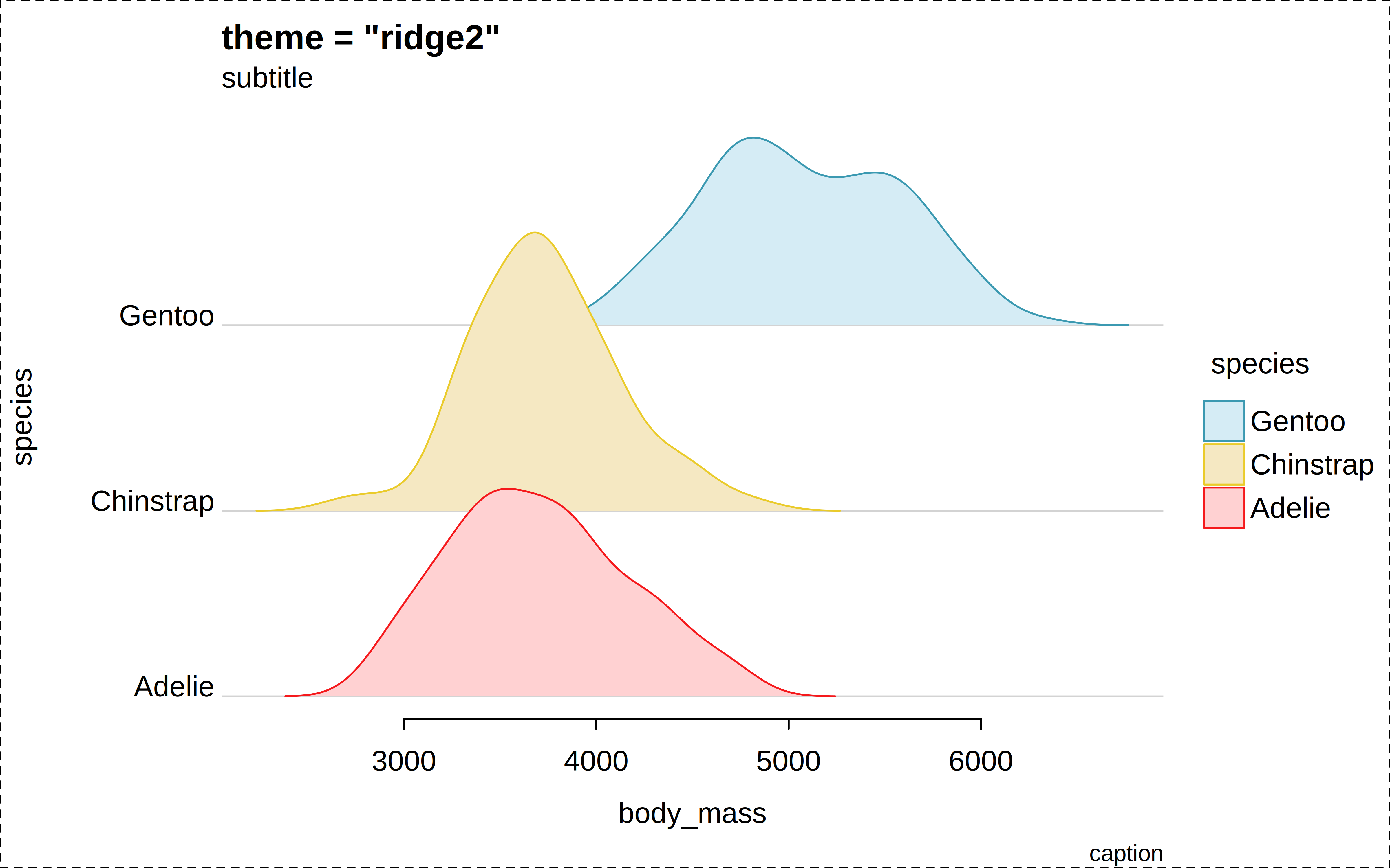
Please feel free to make suggestions about themes, or contribute new themes by opening a Pull Request on Github.
Creating custom tinyplot themes is easy. In this section, we demonstrate how to tweak aexisting themes in an ad hoc manner, as well as how to register your own custom themes for convenient re-use.
The tinytheme() function accepts all of the graphical parameters supported by (t)par(). This means that you customize a persistent theme simply by passing down the relevant parameter arguments. For example:
tinytheme(
"dynamic",
cex = 1.2, cex.main = 1.5,
col.axis = "darkred", col.main = "firebrick",
family = "HersheySans",
grid = TRUE, grid.col = "thistle",
pch = 2
)
tinyplot(mpg ~ hp, data = mtcars, main = "Fuel efficiency vs. horsepower")
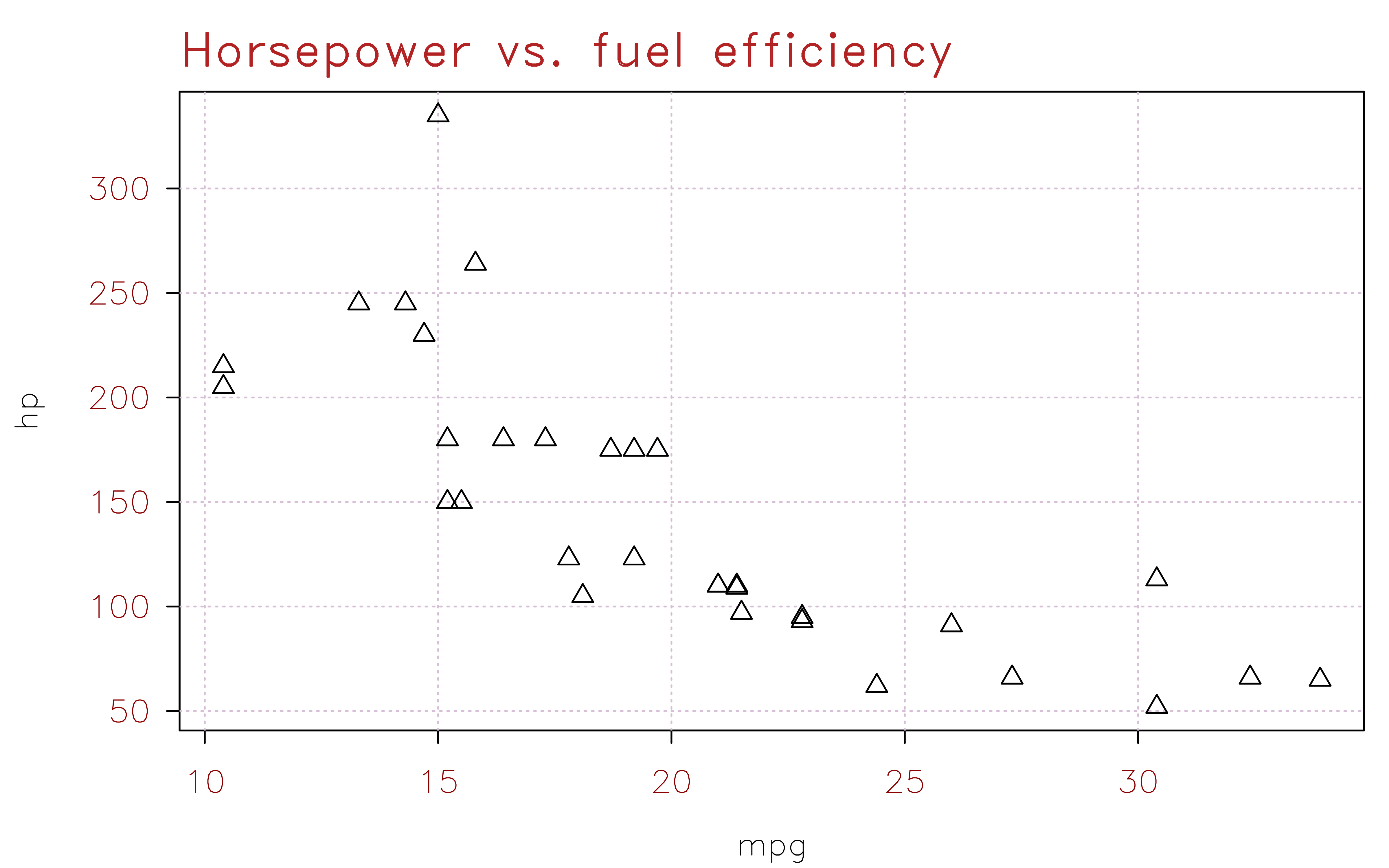
tinyplot(hp ~ mpg, data = mtcars, main = "Horsepower vs. fuel efficiency")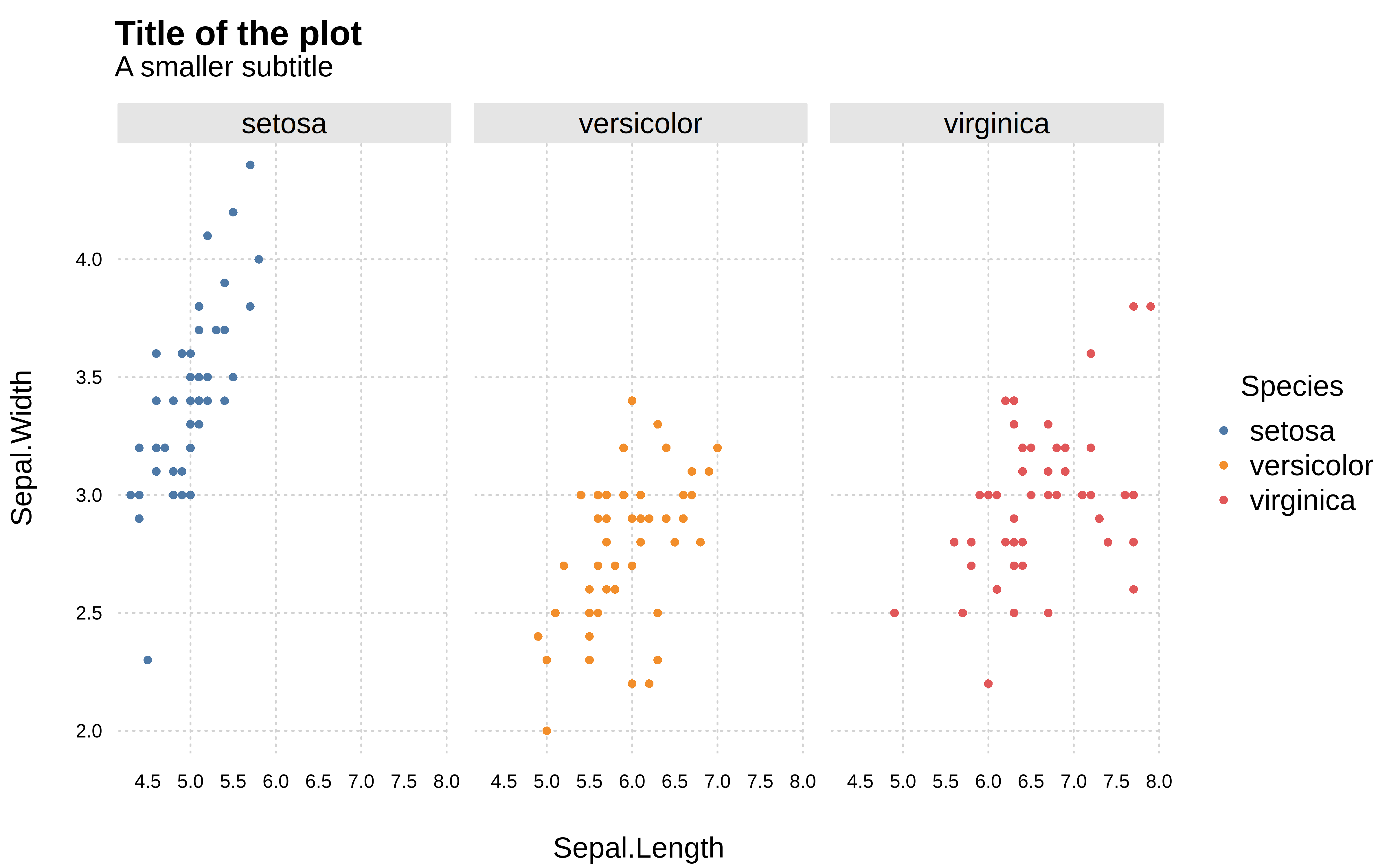
# reset
tinytheme()
Similarly, you can pass a list object to the themes argument to customize an ephemeral theme for a single plot. Here’s a more fancy adaptation that builds off the “dynamic” theme.
tinyplot(
  lat ~ long | depth, data = quakes,
  main = "Earthquakes off Fiji",
  xlab = "Longitutde",
  ylab = "Latitude",
  cap = "Data courtesy of the Harvard PRIM-H project",
  palette = "mako",
  # custom ephemeral theme
  theme = list(
    "dynamic",
    bty = "n",
    bg = "#E0D9D2",
    cex = 1.2, cex.main = 1.5, cex.lab = 1.2,
    col = "#3D3532",
    family = "HersheyScript",
    grid = TRUE, grid.col = "gray95", grid.lwd = 1.5
  )
)
If you find yourself reusing the same custom theme settings across multiple plots or sessions, you may prefer to register them as a named theme with tinytheme_register(). Once a theme is registered, it works just like a built-in one. So you can set it persistently with tinytheme(<yourtheme>), or pass it ephemerally with tinyplot(..., theme = <yourtheme>).
Here’s a (possibly ill-advised) example of a “pirate”-inspired theme:
# Register a custom "pirate" theme that builds on top of "clean"
tinytheme_register(
  "pirate",
  theme = "clean",
  family = "HersheyScript",
  bg = "#f5e6c8", fg = "#3b2209",
  cex.lab = 1.5, cex.main = 1.5, cex.sub = 1.2,
  col = "#3b2209", col.axis = "#5c3a1e", col.cap = "#7a5230",
  col.lab = "#3b2209", col.main = "#1a0f04", col.sub = "#7a5230",
  grid = TRUE, grid.col = "#c9a96e", grid.lty = "dotted",
  facet.bg = "#e8d4a8", facet.border = "#5c3a1e",
  pch = 4,
  palette.qualitative = c(
    "#8b0000", "#1a5276", "#196f3d", "#7d6608",
    "#6c3483", "#a04000", "#1b4f72", "#145a32"
  )
)

# Use it ephemerally
tinyplot(
  Sepal.Length ~ Petal.Length | Species, iris,
  main = 'Avast, me hearties!',
  sub  = 'Here be a "pirate" theme',
  cap  = '"x" marks the spot',
  theme = 'pirate'
)
As a convenience, tinytheme() also accepts a register argument that registers and activates the theme in a single call:
# Equivalent to tinytheme_register("float2", ...) + tinytheme("float2")
tinytheme("float", grid = TRUE, register = "float2")
You can use tinytheme_list() to see all available themes (both built-in and registered), and tinytheme_unregister() to remove one.
tinytheme_unregister("pirate")Note that registered themes are session-scoped: they persist across plots but disappear when R restarts. To make a custom theme permanently available, register it in your .Rprofile:
# In ~/.Rprofile
if (requireNamespace("tinyplot", quietly = TRUE)) {
  tinyplot::tinytheme_register("my_theme", theme = "clean", grid.col = "pink")
}
Similarly, package authors can ship their own custom (tiny)themes as part of their codebase, which any subsequent tinyplot() calls can plug into.
Fonts are a suprisingly effective way to add impact and personality to your plots. While it is perhaps underappreciated, base R actually ships with built-in support for quite a few font families. In the code chunks above we used a member of the Hershey font family that comes bundled with the base R distribution (see ?Hershey). But this built-in support also extends to other popular LaTex and PDF fonts like “Palatino”, “ComputerModern”, “Helvetica”, “AvantGarde”, etc. (see ?pdfFonts).
For access to a much wider variety of fonts, you might consider the excellent showtext package (link). This package allows you to install any font family from the Google Font catalog, either on-the-fly or downloaded to your permanent fontbook collection. It plays very nicely with tinyplot.
One feature of the tinytheme() infrastructure that is especially relevant to customized themes is how dynamic spacing works. Dynamic themes in tinyplot automatically compute margin positions (mar, mgp) so that axis and text elements are well-spaced. Moreover, rather than requiring you to manually reason about how mar, mgp, and tcl combine to produce certain spacing, which—trust us—is both confusing and error prone, you can control the gaps between elements directly through two spacing “primitives”:
gap.axis: the gap (in margin lines) between the tick tip and the near edge of the tick label. Default 0.2.gap.lab: the gap (in margin lines) between the far edge of the tick label and the near edge of the axis title. Default 1.0.These scale automatically with companion features like cex.axis and cex.lab, maintaining constant visible spacing regardless of text size. For example:
tinytheme("dynamic", gap.axis = 0, gap.lab = 0.5)
tinyplot(mpg ~ hp, data = mtcars, main = "Tighter axis gaps")
box("outer", lty = 2)
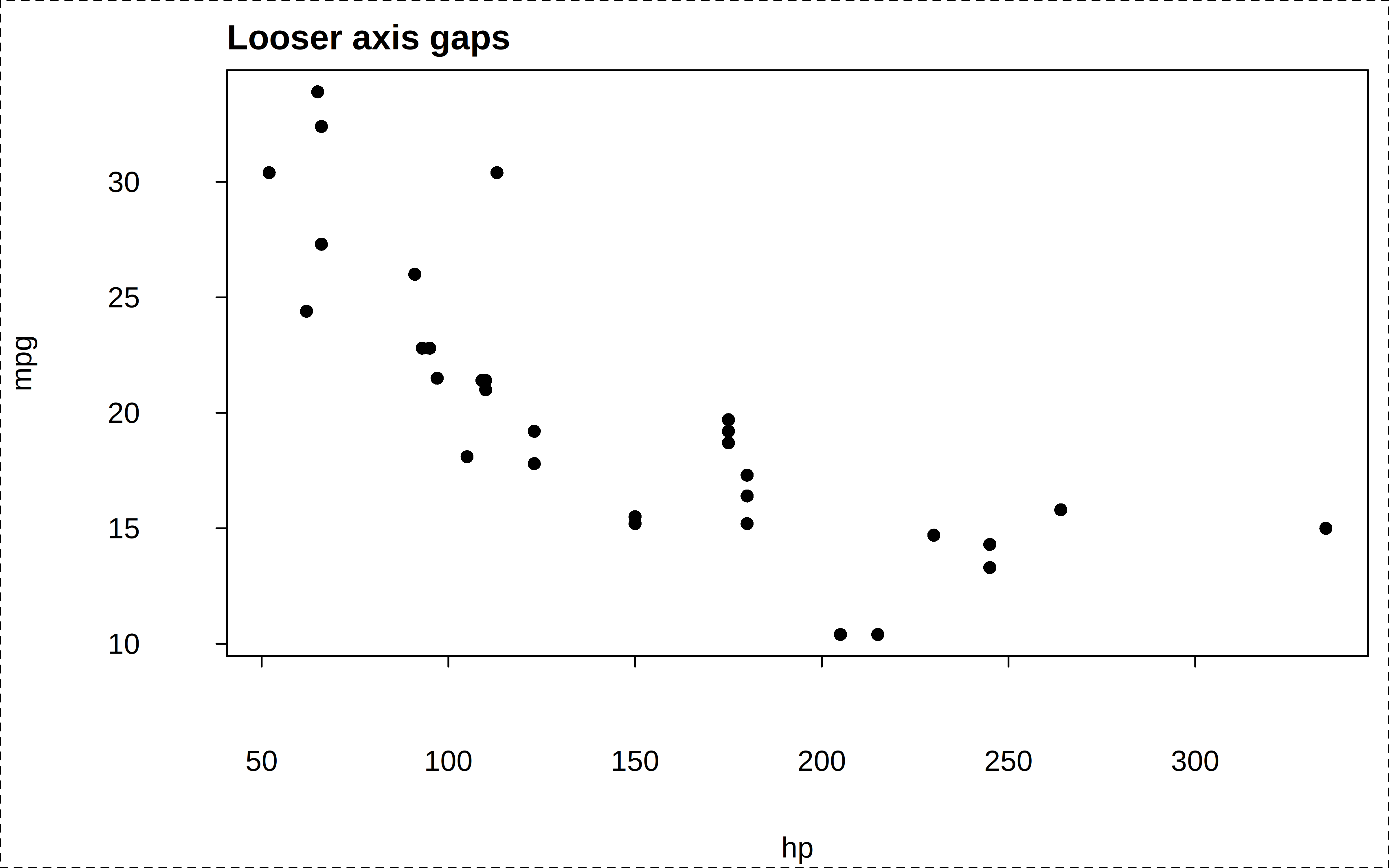
tinytheme("dynamic", gap.axis = 2, gap.lab = 2)
tinyplot(mpg ~ hp, data = mtcars, main = "Looser axis gaps")
box("outer", lty = 2)
tinytheme() # reset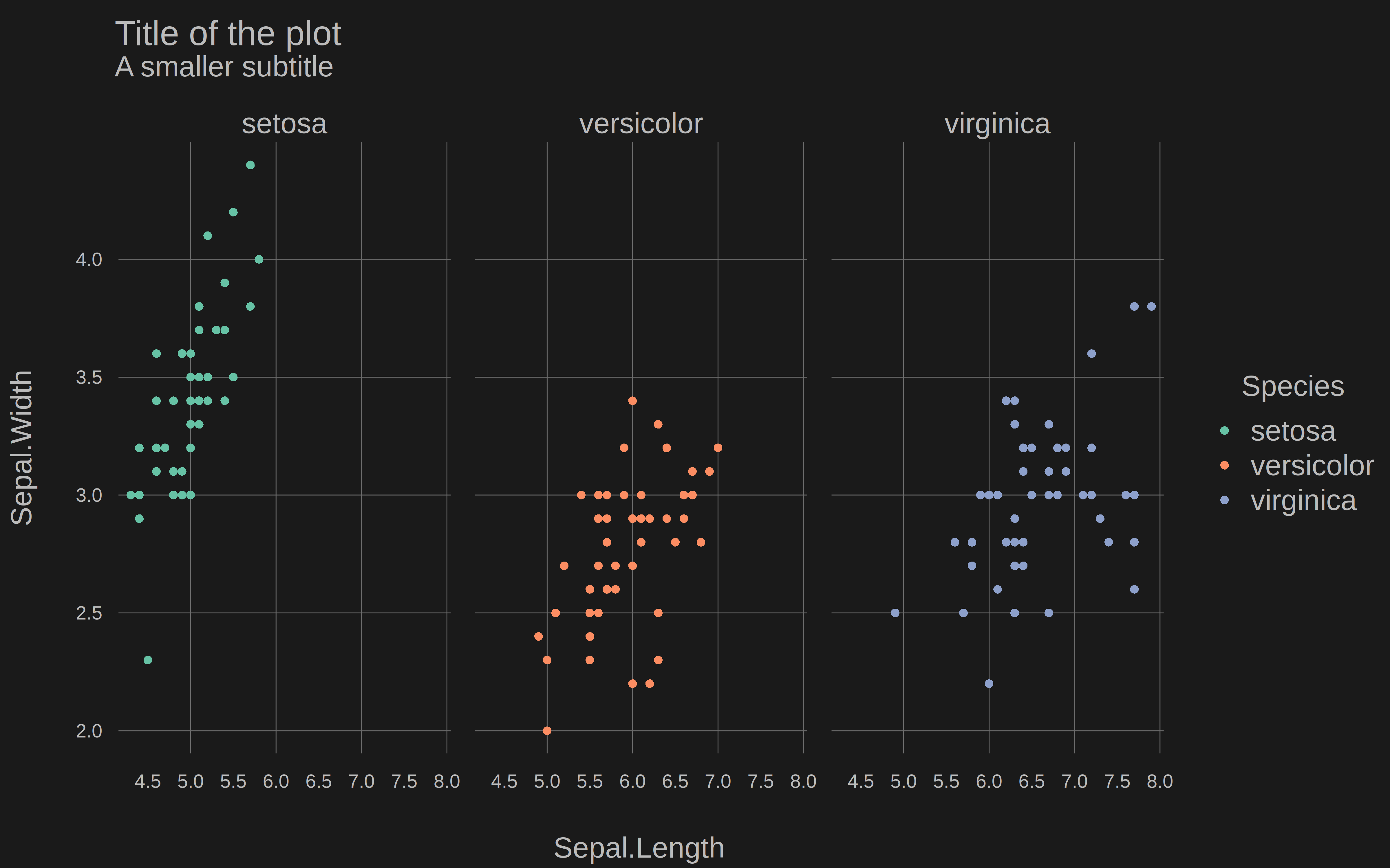
Again, this is much more convenient that fiddling with mgp values. But you can always provide mgp values if you wish; in which it will take precedence and the primitives are ignored.
To see the full list of parameters that defines a particular theme, simply assign them to an object. This can be helpful if you want to explore creating your own custom theme, or tweak an existing theme.
# parms = tinytheme("clean")   # assigns the theme at the same time
parms = tinyplot:::theme_clean # doesn't assign the theme

# show the list of parameters used in the "clean" theme
parms
As a final note about customizing themes, please note that tinytheme works by setting a persistent hook that resets parameters before each new plot. This is an efficient design choice, but it also means that calling (t)par(<params>) on top of an active theme won’t work. This is because the active theme’s hook will override your additional parameter tweaks during the creation of the next plot. All of which is to emphasize that you should pass any theme customizations directly to tinytheme():
# This won't work as expected:
tinytheme("clean")
tpar(mar = c(5, 5, 2, 2))  # overwritten by the theme hook
<some plot>

# Do this instead:
tinytheme("clean", mar = c(5, 5, 2, 2))
<some plot>tpar()Subtitle: And comparison with par()
Themes are a powerful and convenient way to customize your plots. But they are not the only game in town. As any base R plotter would tell you, another way to customize your plots by setting global graphics parameters via par(). If you prefer this approach, then the good news is that it is fully compatable with tinyplot.1 However, we recommend that you rather use tpar(), which is an extended version of par() that supports all of the latter’s parameters plus some tinyplot-specific upgrades.
Here is a quick example, where we impose several global changes (e.g., change the font family, use Tufte-style floating axes with a background panel grid, rotate tick labels, etc.) before drawing the plot.
op = tpar(
  bty    = "n",           # No box (frame) around the plot
  family = "HersheySans", # Use R's Hershey font instead of Arial default
  grid   = TRUE,          # Add a background grid
  las    = 1,             # Horizontal axis tick labels
  pch    = 19             # Larger filled points as default
)

tinyplot(Sepal.Length ~ Petal.Length | Species, data = iris, alpha = 0.5)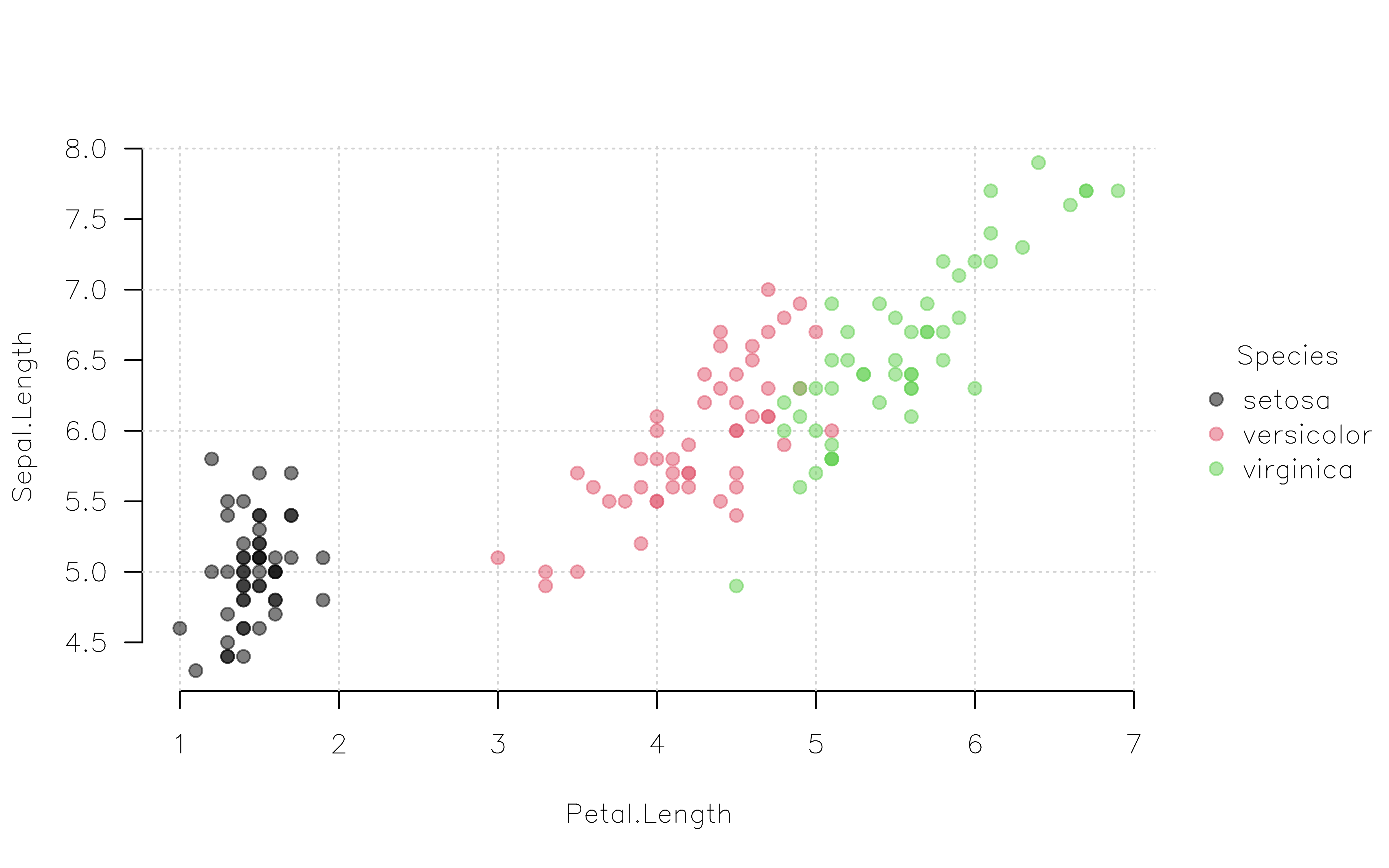
# optional: reset to the original parameter settings
tpar(op)
Again, this approach should feel very familiar to experience base R plotters. But we will drive home the point by exploring one final difference between vanilla par() and the enhanced tpar() equivalent…
The graphical parameters set by par() stay in force as long as a graphical device stays open. On the other hand, these parameters are reset when the plotting window is closed or, for example, when executing a new code chunk in a Quarto notebook.2
par(col = "red", pch = 4)
tinyplot(mpg ~ hp, data = mtcars)
tinyplot(wt ~ qsec, data = mtcars)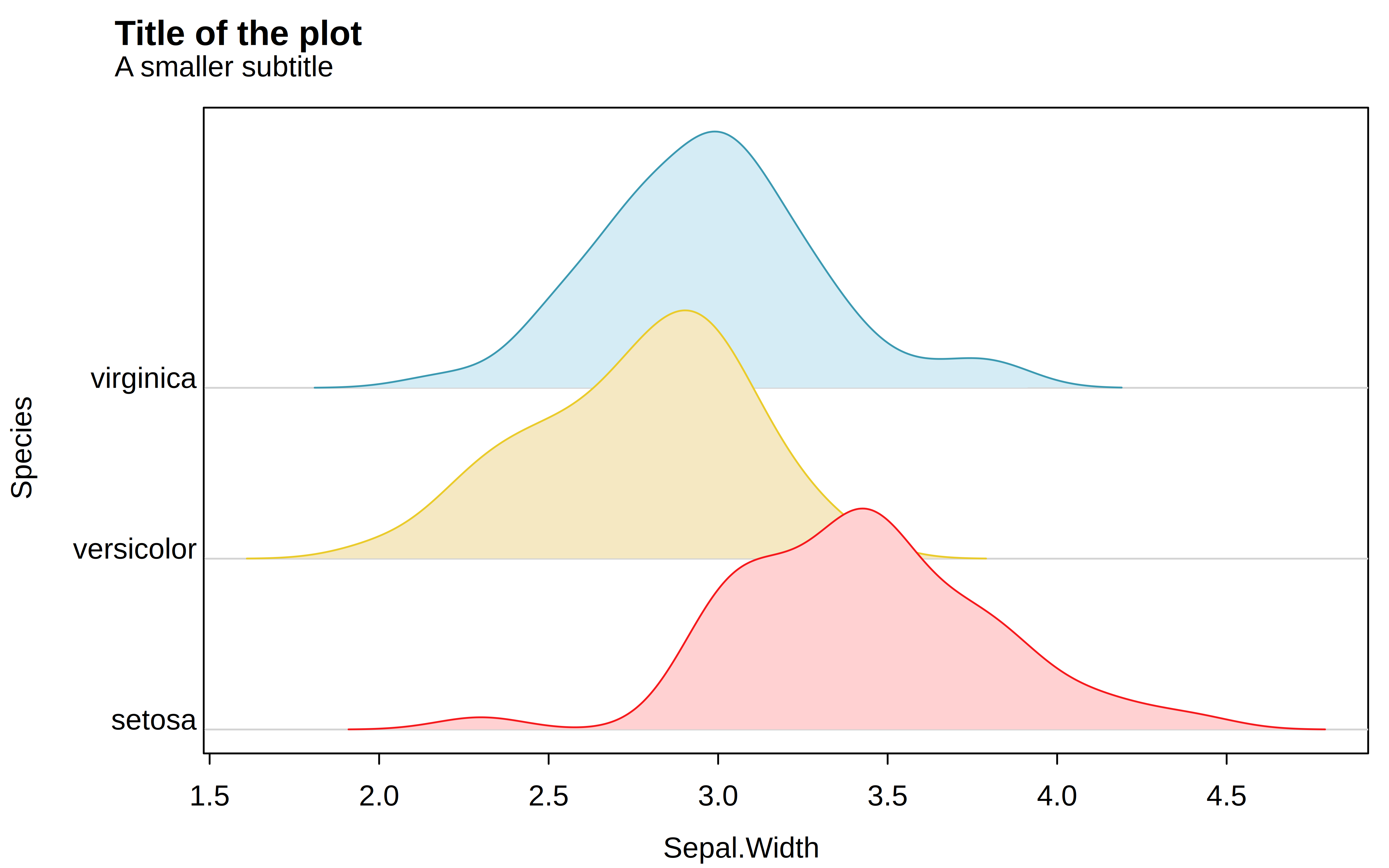
In contrast, graphical parameters set by tpar() can persist across devices and Quarto code chunks thanks to a built-in “hook” mechanism (see ?setHook). To enable this persistence, we must invoke the hook=TRUE argument.
tpar(col = "red", pch = 4, hook = TRUE)
tinyplot(mpg ~ hp, data = mtcars)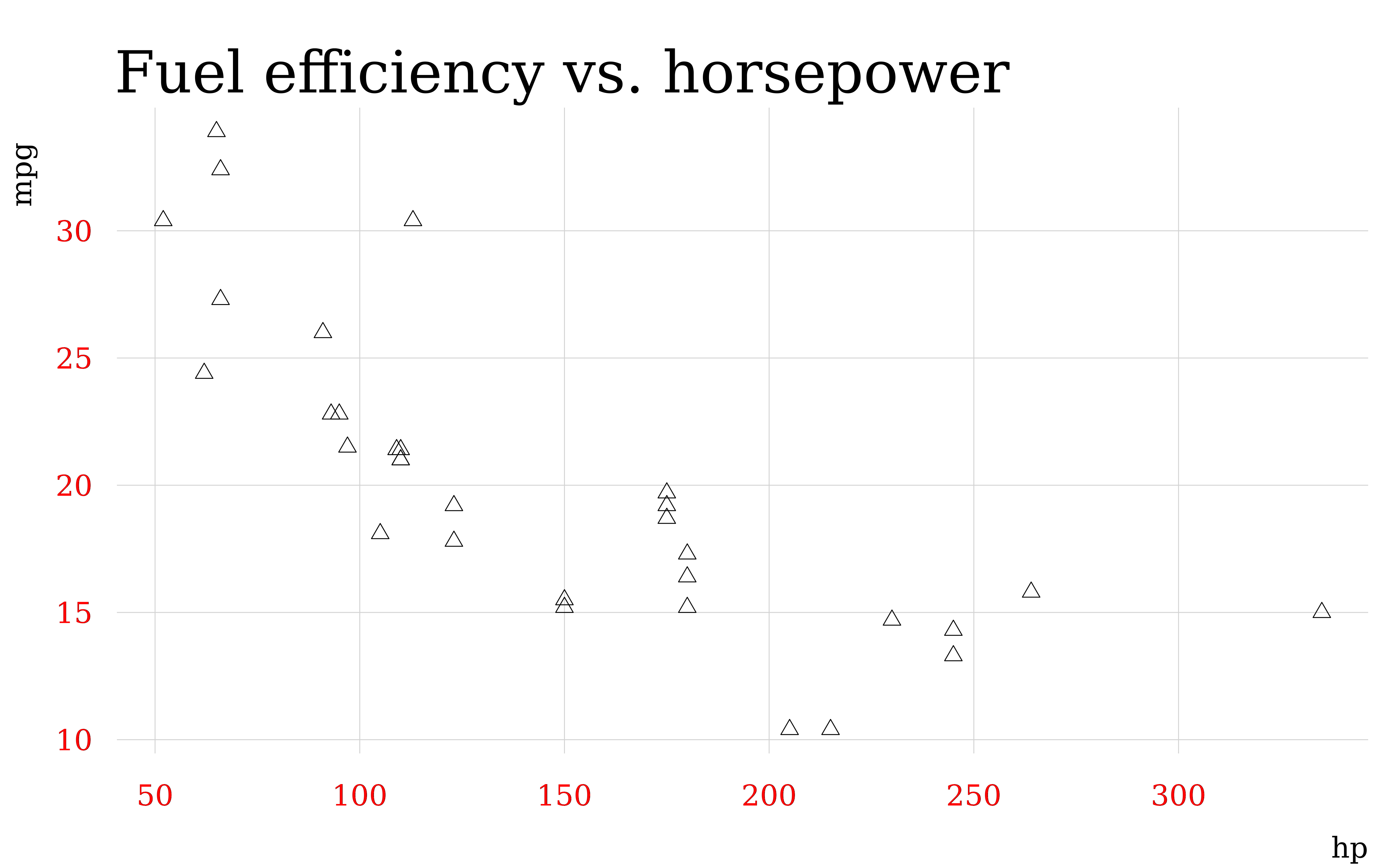
tinyplot(wt ~ qsec, data = mtcars)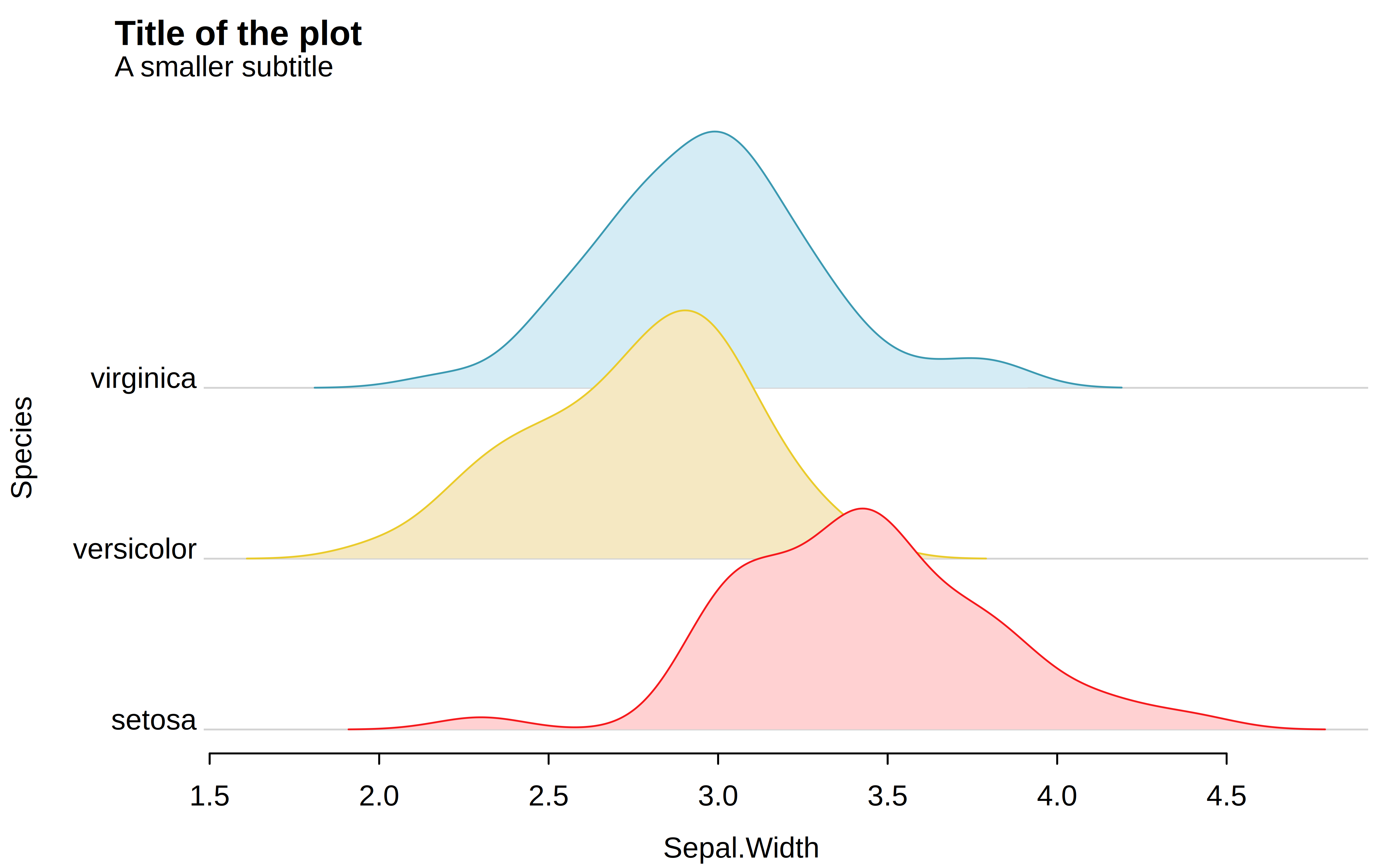
# reset defaults
tinytheme()
(Fun fact: Behind the scenes, tinytheme(<theme_name>) is simply passing a list of parameters to tpar(..., hook = TRUE).)
After all, a tinyplot is just a base plot with added convenience features. We still use the same graphics engine under the hood and any settings and workflows for plot() should (ideally) carry over to tinyplot() too.↩︎
The knitr package, which provides the rendering engine for Quarto and R Markdown, also has a global.par option to overcome this limitation. See here.↩︎