x, y
|
the x and y arguments provide the x and y coordinates for the plot. Any reasonable way of defining the coordinates is acceptable; most likely the names of existing vectors or columns of data frames. See the ‘Examples’ section below, or the function xy.coords for details. If supplied separately, x and y must be of the same length.
|
…
|
other graphical parameters. If type is a character specification (such as “hist”) then any argument names that match those from the corresponding type_*() function (such as type_hist) are passed on to that. All remaining arguments from … can be further graphical parameters, see par).
|
xmin, xmax, ymin, ymax
|
minimum and maximum coordinates of relevant area or interval plot types. Only used when the type argument is one of “rect” or “segments” (where all four min-max coordinates are required), or “pointrange”, “errorbar”, or “ribbon” (where only ymin and ymax required alongside x). Can be passed as unquoted (NSE) variable names when called from the tinyplot.formula method, e.g. ymin = varname where varname is a variable in data.
|
weights
|
an optional numeric vector of observation weights, of the same length as the number of x,y coordinates. Can be passed as an unquoted (NSE) variable name when called from the tinyplot.formula method, e.g. weights = varname where varname is a variable in data. Weights are only consumed by the plot types that support them; specifically, the model fit and distribution types like type_lm() and type_spineplot(). Because weights trigger a statistical transformation, a warning is emitted if this argument is supplied to a non-supported type (even though the actual weights will be ignored, regardless).
|
labels
|
an optional vector of text labels for use with type_text(), of length 1 or the same length as the number of x,y coordinates. Can be passed as an unquoted (NSE) variable name when called from the tinyplot.formula method, e.g. labels = varname where varname is a variable in data. Ignored by other plot types. Overrides the labels argument of type_text() if both are supplied.
|
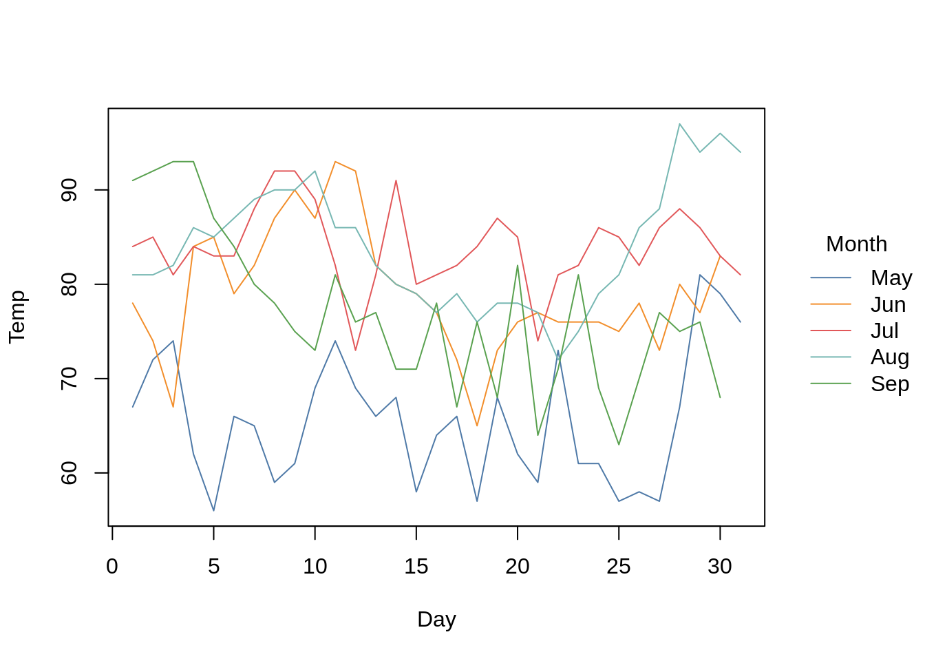
by
|
grouping variable(s). The default behaviour is for groups to be represented in the form of distinct colours, which will also trigger an automatic legend. (See legend below for customization options.) However, groups can also be presented through other plot parameters (e.g., pch, lty, or cex) by passing an appropriate “by” keyword; see Examples. Note that continuous (i.e., gradient) colour legends are also supported if the user passes a numeric or integer to by. To group by multiple variables, wrap them with interaction.
|
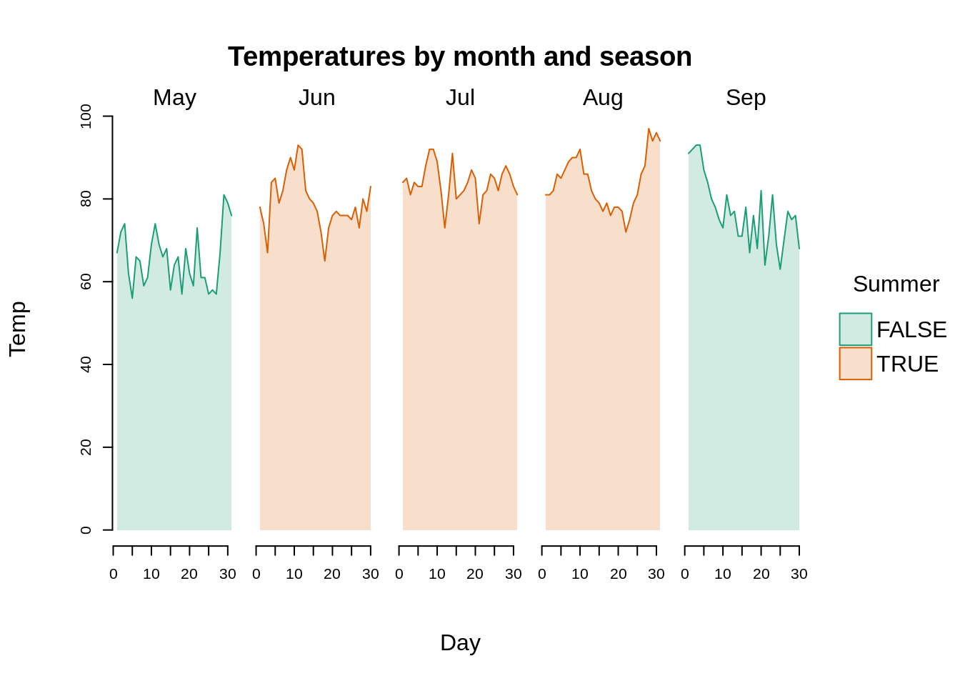
facet
|
the faceting variable(s) that you want arrange separate plot windows by. Can be specified in various ways:
-
In "atomic" form, e.g. facet = fvar. To facet by multiple variables in atomic form, simply interact them, e.g. interaction(fvar1, fvar2) or factor(fvar1):factor(fvar2).
-
As a one-sided formula, e.g. facet = ~fvar. Multiple variables can be specified in the formula RHS, e.g. ~fvar1 + fvar2 or ~fvar1:fvar2. Note that these multi-variable cases are all treated equivalently and converted to interaction(fvar1, fvar2, …) internally. (No distinction is made between different types of binary operators, for example, and so f1+f2 is treated the same as f1:f2, is treated the same as f1*f2, etc.)
-
As a two-side formula, e.g. facet = fvar1 ~ fvar2. In this case, the facet windows are arranged in a fixed grid layout, with the formula LHS defining the facet rows and the RHS defining the facet columns. At present only single variables on each side of the formula are well supported. (We don’t recommend trying to use multiple variables on either the LHS or RHS of the two-sided formula case.)
-
As a special “by” convenience keyword, in which case facets will match the grouping variable(s) passed to by above.
|
facet.args
|
an optional list of arguments for controlling faceting behaviour. (Ignored if facet is NULL.) Supported arguments are as follows:
-
nrow, ncol for overriding the default "square" facet window arrangement. Only one of these should be specified, but nrow will take precedence if both are specified together. Ignored if a two-sided formula is passed to the main facet argument, since the layout is arranged in a fixed grid.
-
free a logical value indicating whether the axis limits (scales) for each individual facet should adjust independently to match the range of the data within that facet. Default is FALSE. Separate free scaling of the x- or y-axis (i.e., whilst holding the other axis fixed) is not currently supported.
-
fmar a vector of form c(b,l,t,r) for controlling the base margin between facets in terms of lines. Defaults to the value of tpar(“fmar”), which should be c(1,1,1,1), i.e. a single line of padding around each individual facet, assuming it hasn’t been overridden by the user as part their global tpar settings. Note some automatic adjustments are made for certain layouts, and depending on whether the plot is framed or not, to reduce excess whitespace. See tpar for more details.
-
cex, font, col, bg, border for adjusting the facet title text and background. Default values for these arguments are inherited from tpar (where they take a "facet." prefix, e.g. tpar(“facet.cex”)). The latter function can also be used to set these features globally for all tinyplot plots.
|
data
|
a data.frame (or list) from which the variables in formula should be taken. A matrix is converted to a data frame.
|
type
|
character string or call to a type_*() function giving the type of plot desired.
-
NULL (default): Choose a sensible type for the type of x and y inputs (i.e., usually “p”).
-
1-character values supported by plot:
-
“p” Points
-
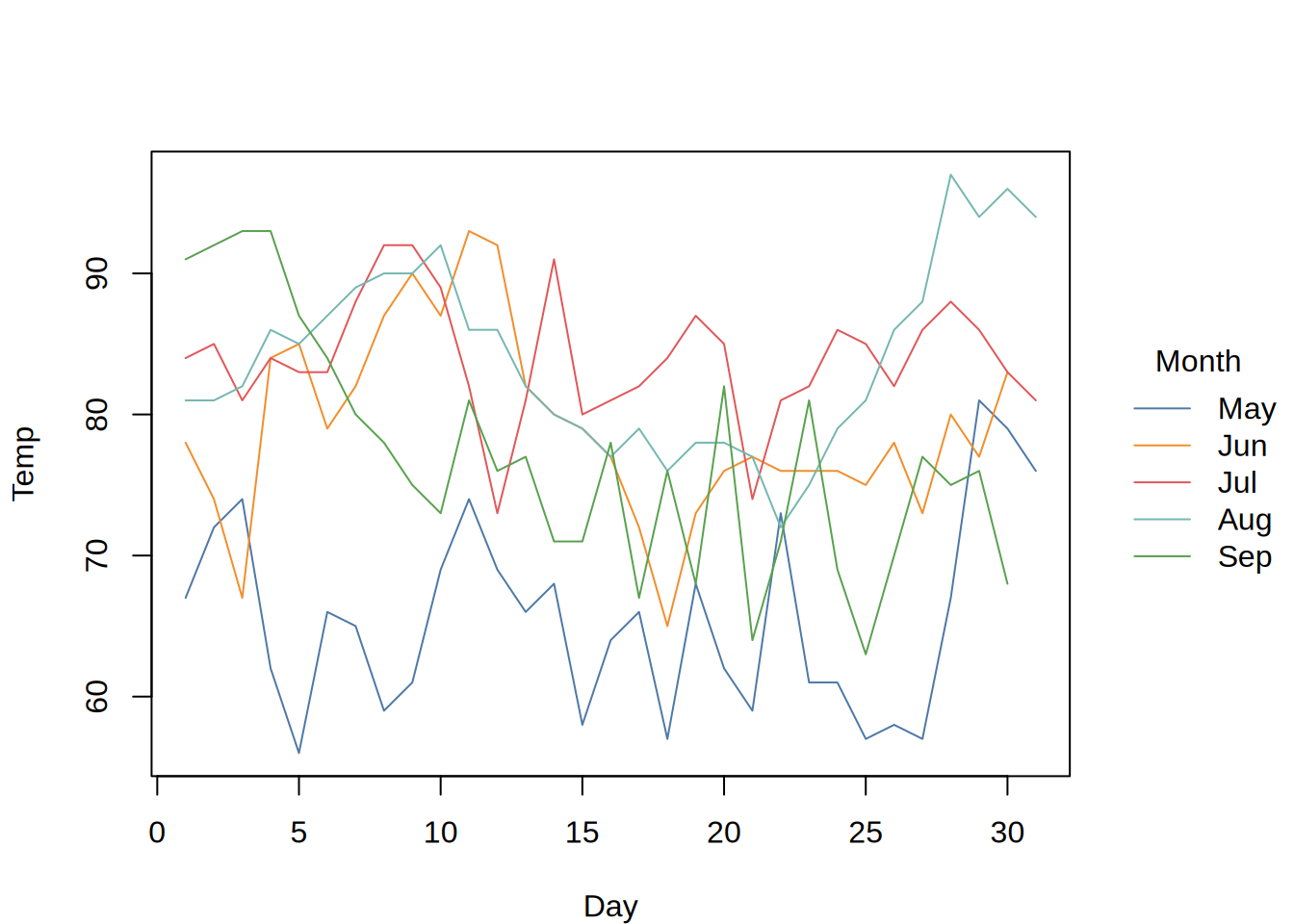
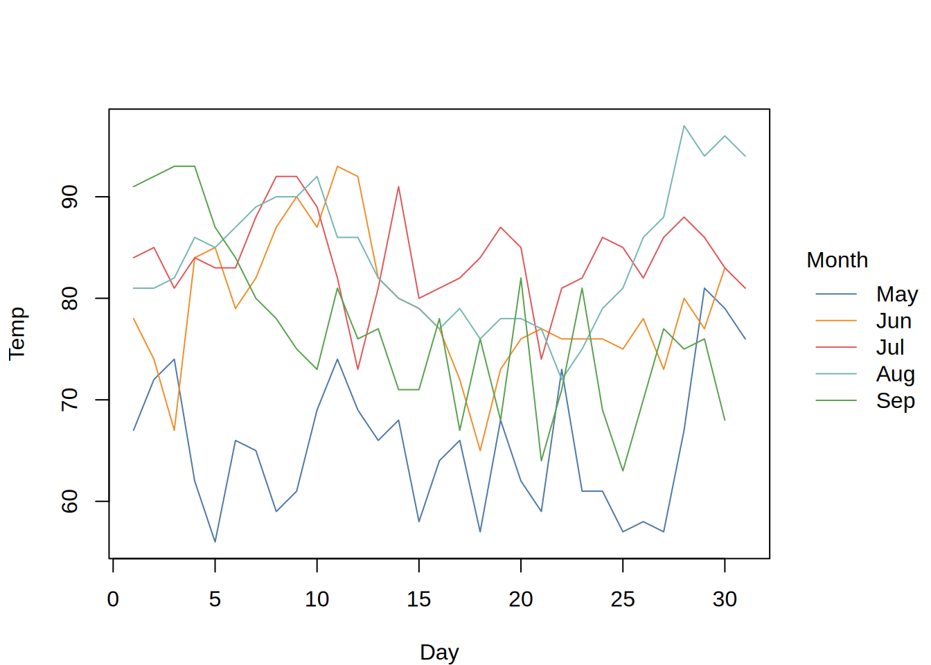
“l” Lines
-
“b” Both points and lines
-
“c” Empty points joined by lines
-
“o” Overplotted points and lines
-
“s” Stair steps
-
“S” Stair steps
-
“h” Histogram-like vertical lines
-
“n” Empty plot over the extent of the data
-
tinyplot-specific types. These fall into several categories:
-
Shapes:
-
“area” / type_area(): Plots the area under the curve from y = 0 to y = f(x).
-
“errorbar” / type_errorbar(): Adds error bars to points; requires ymin and ymax.
-
“pointrange” / type_pointrange(): Combines points with error bars.
-
“polygon” / type_polygon(): Draws polygons.
-
“polypath” / type_polypath(): Draws a path whose vertices are given in x and y.
-
“rect” / type_rect(): Draws rectangles; requires xmin, xmax, ymin, and ymax.
-
“ribbon” / type_ribbon(): Creates a filled area between ymin and ymax.
-
“segments” / type_segments(): Draws line segments between pairs of points.
-
“text” / type_text(): Add text annotations.
-
Visualizations:
-
“barplot” / type_barplot(): Creates a bar plot.
-
“boxplot” / type_boxplot(): Creates a box-and-whisker plot.
-
“chull” / type_chull(): Draws convex hull(s) around grouped points.
-
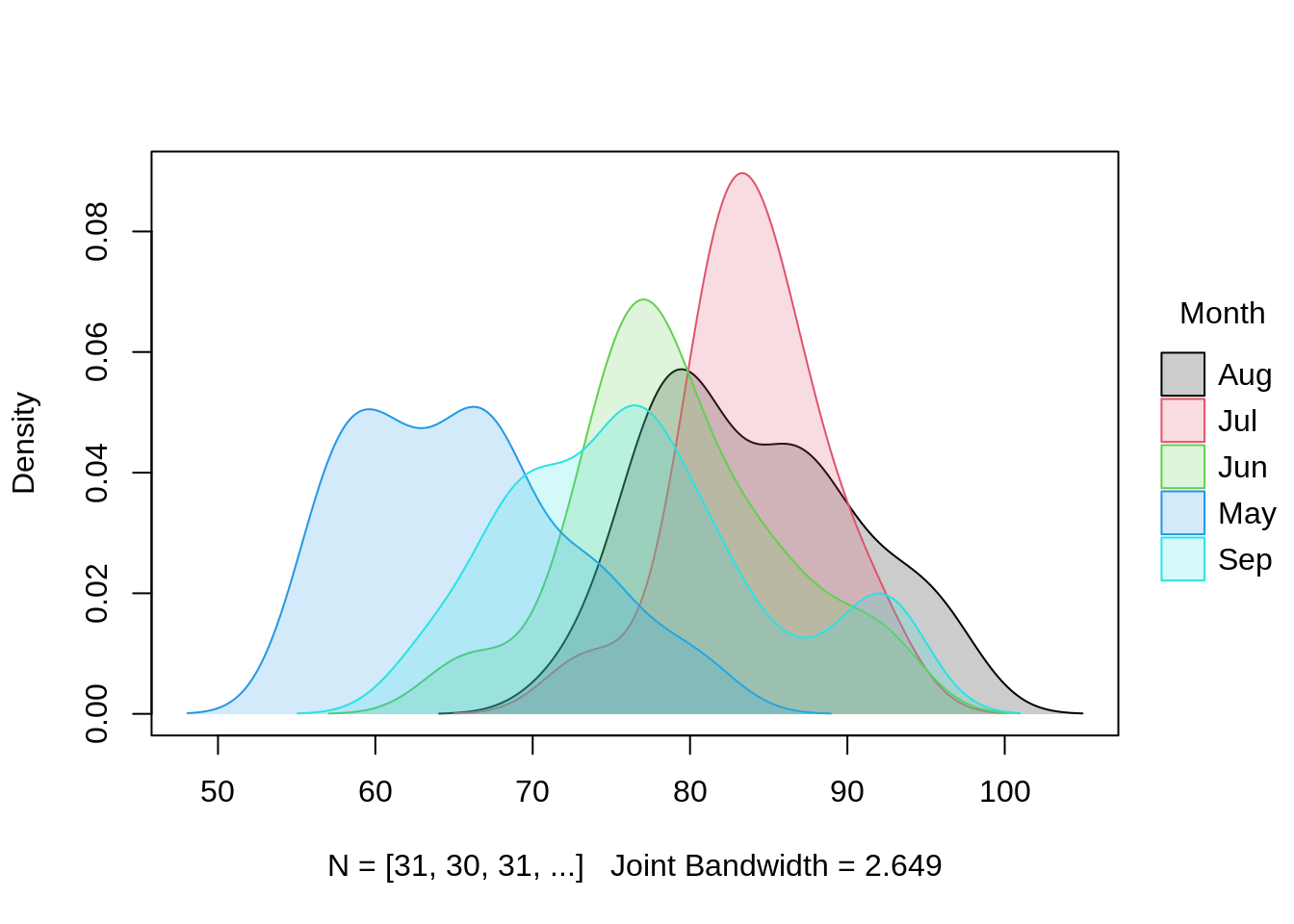
“density” / type_density(): Plots the density estimate of a variable.
-
“histogram” / type_histogram(): Creates a histogram of a single variable.
-
“jitter” / type_jitter(): Jittered points.
-
“qq” / type_qq(): Creates a quantile-quantile plot.
-
“ridge” / type_ridge(): Creates a ridgeline (aka joy) plot.
-
“rug” / type_rug(): Adds a rug to an existing plot.
-
“spineplot” / type_spineplot(): Creates a spineplot or spinogram.
-
“violin” / type_violin(): Creates a violin plot.
-
Models:
-
“loess” / type_loess(): Local regression curve.
-
“lm” / type_lm(): Linear regression line.
-
“glm” / type_glm(): Generalized linear model fit.
-
“spline” / type_spline(): Cubic (or Hermite) spline interpolation.
-
Functions:
-
type_abline(): line(s) with intercept and slope.
-
type_hline(): horizontal line(s).
-
type_vline(): vertical line(s).
-
type_function(): arbitrary function.
-
type_summary(): summarize y by unique values of x.
|
legend
|
one of the following options:
-
NULL (default), in which case the legend will be determined by the grouping variable. If there is no group variable (i.e., by is NULL) then no legend is drawn. If a grouping variable is detected, then an automatic legend is drawn to the outer right of the plotting area. Note that the legend title and categories will automatically be inferred from the by argument and underlying data.
-
A convenience string indicating the legend position. Supported keywords:
-
Standard position keywords from base legend(), e.g. “right”, “topleft”, “bottom”, etc.
-
Outer positions via a trailing “!”, e.g. “right!”, “topleft!”, or “bottom!”. This places the legend outside the plotting area and adjusts the margins accordingly.
-
“direct”: places text labels at the last point of each group’s data, coloured to match. Best suited to line-based plots with x-sorted data, where "last" corresponds to "rightmost". The right margin is automatically expanded to prevent clipping. Requires discrete groups via by. For faceted plots, labels are drawn in each panel for the groups present there. Supports additional arguments when passed via legend(…):
-
nudge_x, nudge_y: numeric vectors of per-group offsets in data units. Recycled to the number of groups. Supports named vectors for targeted adjustment, e.g. nudge_y = c(“Group A” = -10, “Group B” = 20).
-
repel: if TRUE, automatically separates overlapping labels vertically. If a positive number, sets the minimum gap between labels in data units.
-
“none”: turns off legend printing.
-
Logical value, where TRUE corresponds to the default case above (same effect as specifying NULL) and FALSE turns the legend off (same effect as specifying "none").
-
A list or, equivalently, a dedicated legend() function with supported legend arguments, e.g. "bty", "horiz", and so forth. To suppress the legend title, set title = NULL or title = FALSE, e.g. legend = list(title = FALSE).
|
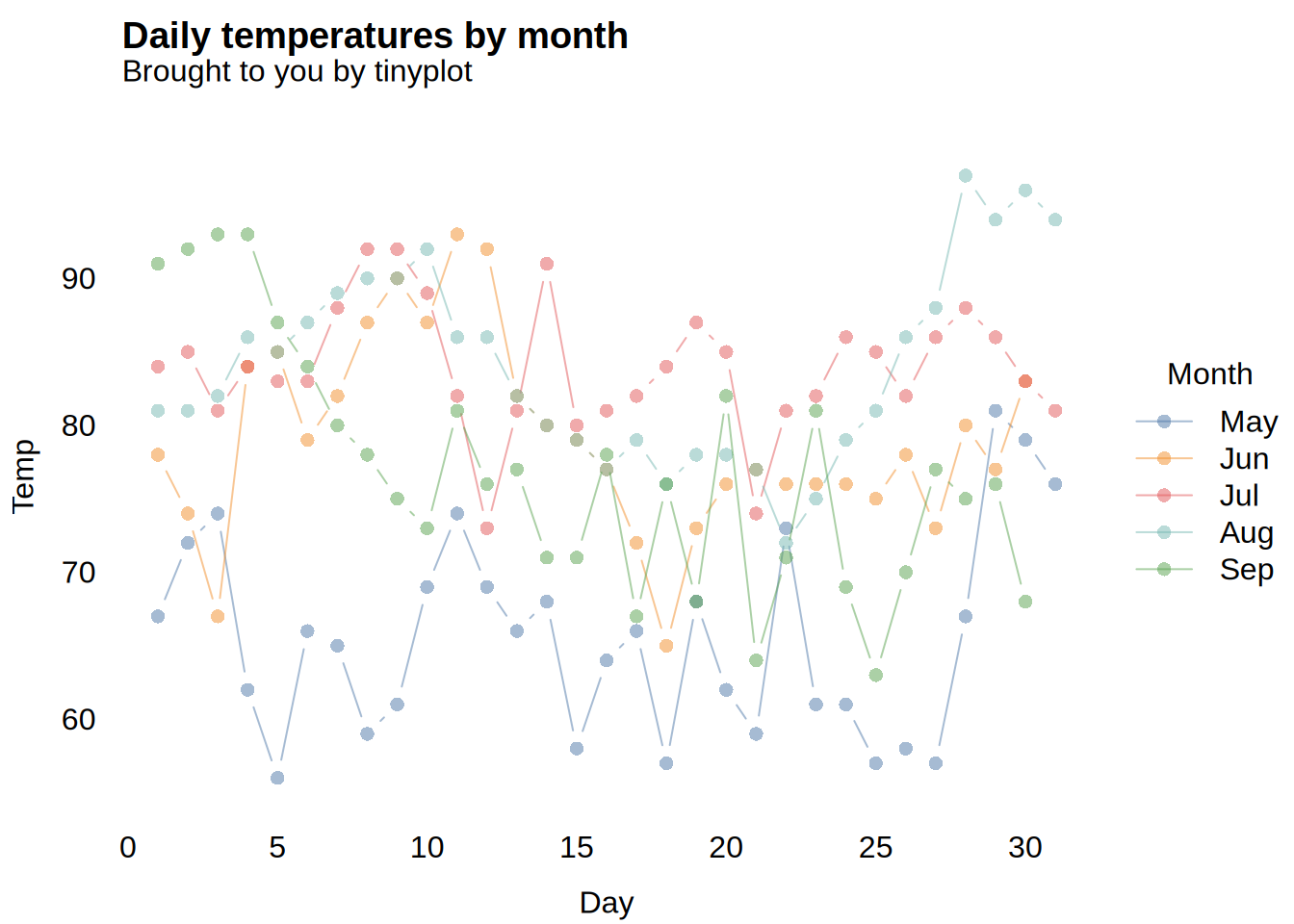
main
|
a main title for the plot, see also title.
|
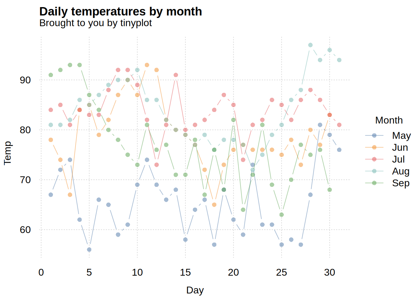
sub
|
a subtitle for the plot.
|
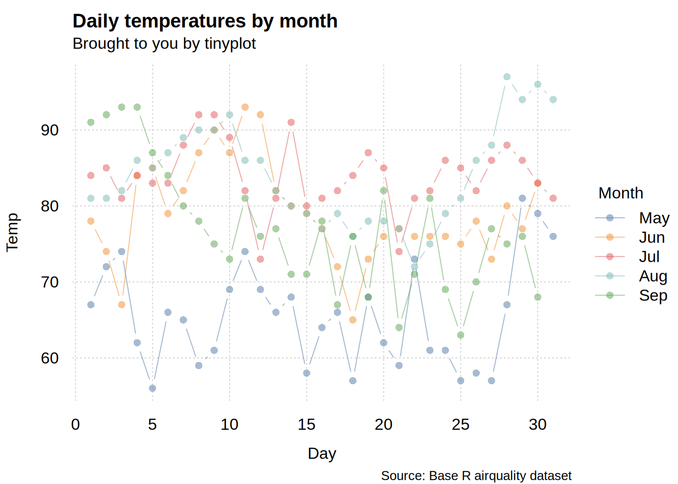
cap
|
a caption for the plot, drawn at the bottom. Useful for annotations like data sources. Best paired with a dynamic tinytheme. For the default theme, should be seen as a substitute for sub, since these two will otherwise overlap. Appearance can be customized via tpar parameters adj.cap, cex.cap, col.cap, font.cap, and line.cap.
|
xlab
|
a label for the x axis, defaults to a description of x.
|
ylab
|
a label for the y axis, defaults to a description of y.
|
ann
|
a logical value indicating whether the default annotation (title and x and y axis labels) should appear on the plot.
|
xlim
|
the x limits (x1, x2) of the plot. Note that x1 > x2 is allowed and leads to a reversed axis (although see the “rev(erse)” keyword option below). The default value, NULL, indicates that the range of the finite values to be plotted should be used. Alongside the standard length-2 vector (e.g., xlim = c(0, 1)), tinyplot supports three further convenience forms:
-
a single scalar (e.g. xlim = 0) ensures that the provided value is covered by the axis range, irrespective of the data extent.
-
a length-2 vector with one NA (e.g. xlim = c(0, NA)) pins the non-NA limit and lets the data determine the other limit.
-
the convenience string “rev” (or the longer “reverse”) reverses the automatically-computed axis range. This is equivalent to passing a descending vector, but without having to know the data extent in advance.
|
ylim
|
the y limits of the plot. Accepts the same input forms as xlim.
|
axes
|
logical or character. Should axes be drawn (TRUE or FALSE)? Or alternatively what type of axes should be drawn: “standard” (with axis, ticks, and labels; equivalent to TRUE), “none” (no axes; equivalent to FALSE), “ticks” (only ticks and labels without axis line), “labels” (only labels without ticks and axis line), “axis” (only axis line and labels but no ticks). To control this separately for the two axes, use the character specifications for xaxt and/or yaxt.
|
xaxt, yaxt
|
character specifying the type of x-axis and y-axis, respectively. See axes for the possible values.
|
xaxs, yaxs
|
character specifying the style of the interval calculation used for the x-axis and y-axis, respectively. See par for the possible values.
|
xaxb, yaxb
|
numeric vector (or character vector, if appropriate) giving the break points at which the axis tick-marks are to be drawn. Break points outside the range of the data will be ignored if the associated axis variable is categorical, or an explicit x/ylim range is given.
|
xaxl, yaxl
|
a function or a character keyword specifying the format of the x- or y-axis tick labels. Note that this is a post-processing step that affects the appearance of the tick labels only; use in conjunction with x/yaxb if you would like to adjust the position of the tick marks too. In addition to user-supplied formatting functions (e.g., format, toupper, abs, or other custom function), several convenience keywords (or their symbol equivalents) are available for common formatting transformations: “percent” (“%”), “comma” (“,”), “log” (“l”), “dollar” (“$”), “euro” (“€”), or “sterling” (“£”). See the tinylabel documentation for examples.
|
log
|
a character string which contains “x” if the x axis is to be logarithmic, “y” if the y axis is to be logarithmic and “xy” or “yx” if both axes are to be logarithmic.
|
flip
|
logical. Should the plot orientation be flipped, so that the y-axis is on the horizontal plane and the x-axis is on the vertical plane? Default is FALSE.
|
frame.plot
|
a logical indicating whether a box should be drawn around the plot. Can also use frame as an acceptable argument alias. The default is to draw a frame if both axis types (set via axes, xaxt, or yaxt) include axis lines.
|
grid
|
argument for plotting a background panel grid, one of:
-
a logical (i.e., TRUE to draw the grid on both axes).
-
a character string controlling which axes get grid lines and at what resolution. Uppercase letters (“X”, “Y”, “XY”) draw grid lines at the standard axis tick positions (with the latter equivalent to TRUE), while lowercase letters (“x”, “y”, “xy”) draw a finer grid with additional lines at the midpoints between ticks. (Note: the finer grid has no effect on log-scale axes, since tick positions already include intermediate values.)
-
a panel grid plotting function like grid(). Note that this argument replaces the panel.first and panel.last arguments from base plot() and tries to make the process more seamless with better default behaviour. The default behaviour is determined by (and can be set globally through) the value of tpar(“grid”).
|
palette
|
one of the following options:
-
NULL (default), in which case the palette will be chosen according to the class and cardinality of the "by" grouping variable. For non-ordered factors or strings with a reasonable number of groups, this will inherit directly from the user’s default palette (e.g., "R4"). In other cases, including ordered factors and high cardinality, the "Viridis" palette will be used instead. Note that a slightly restricted version of the "Viridis" palette—where extreme color values have been trimmed to improve visual perception—will be used for ordered factors and continuous variables. In the latter case of a continuous grouping variable, we also generate a gradient legend swatch.
-
A convenience string corresponding to one of the many palettes listed by either palette.pals() or hcl.pals(). Note that the string can be case-insensitive (e.g., "Okabe-Ito" and "okabe-ito" are both valid).
-
A palette-generating function. This can be "bare" (e.g., palette.colors) or "closed" with a set of named arguments (e.g., palette.colors(palette = “Okabe-Ito”, alpha = 0.5)). Note that any unnamed arguments will be ignored and the key n argument, denoting the number of colours, will automatically be spliced in as the number of groups.
-
A vector or list of colours, e.g. c(“darkorange”, “purple”, “cyan4”). If too few colours are provided for a discrete (qualitative) set of groups, then the colours will be recycled with a warning. For continuous (sequential) groups, a gradient palette will be interpolated.
|
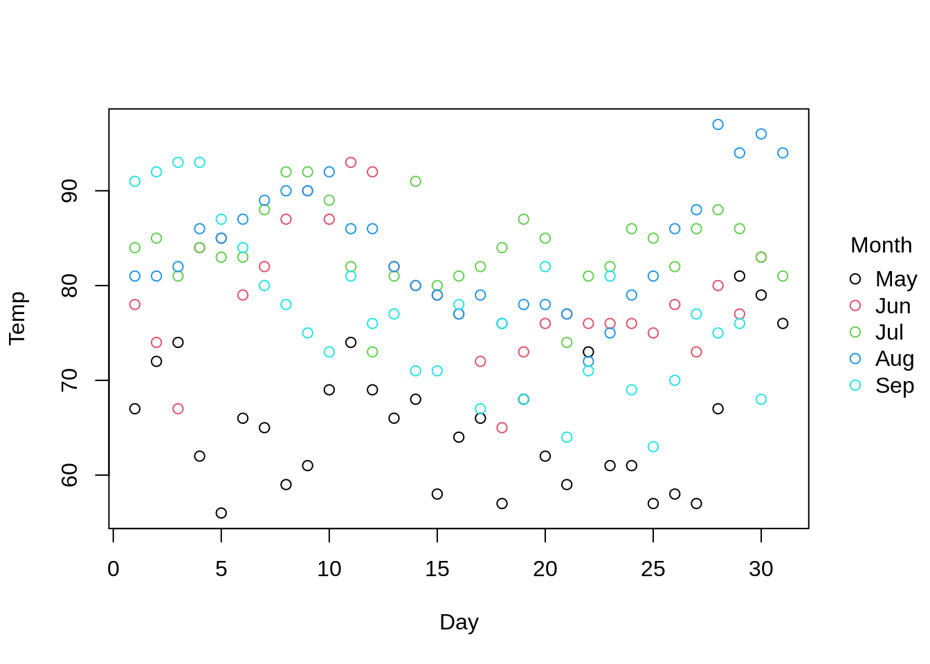
pch
|
plotting "character", i.e., symbol to use. Character, integer, or vector of length equal to the number of categories in the by variable. See pch. In addition, users can supply a special pch = “by” convenience argument, in which case the characters will automatically loop over the number groups. This automatic looping will begin at the global character value (i.e., par(“pch”)) and recycle as necessary.
|
lty
|
line type. Character, integer, or vector of length equal to the number of categories in the by variable. See lty. In addition, users can supply a special lty = “by” convenience argument, in which case the line type will automatically loop over the number groups. This automatic looping will begin at the global line type value (i.e., par(“lty”)) and recycle as necessary.
|
lwd
|
line width. Numeric scalar or vector of length equal to the number of categories in the by variable. See lwd. In addition, users can supply a special lwd = “by” convenience argument, in which case the line width will automatically loop over the number of groups. This automatic looping will be centered at the global line width value (i.e., par(“lwd”)) and pad on either side of that.
|
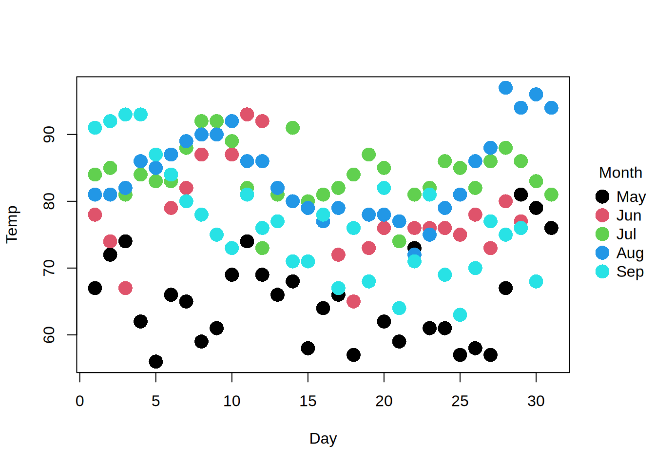
col
|
plotting color. Character, integer, or vector of length equal to the number of categories in the by variable. See col. Note that the default behaviour in tinyplot is to vary group colors along any variables declared in the by argument. Thus, specifying colors manually should not be necessary unless users wish to override the automatic colors produced by this grouping process. Typically, this would only be done if grouping features are deferred to some other graphical parameter (i.e., passing the "by" keyword to one of pch, lty, lwd, or bg; see below.)
|
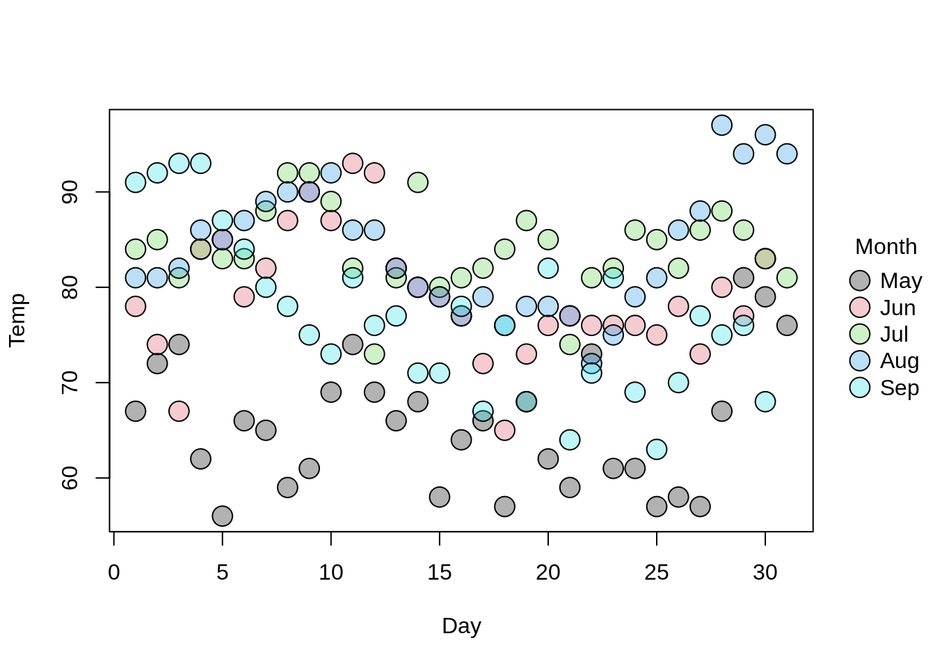
bg
|
background fill color for the open plot symbols 21:25 (see points.default), as well as ribbon and area plot types. Users can also supply either one of two special convenience arguments that will cause the background fill to inherit the automatic grouped coloring behaviour of col:
-
bg = “by” will insert a background fill that inherits the main color mappings from col.
-
by = <numeric[0,1]> (i.e., a numeric in the range [0,1]) will insert a background fill that inherits the main color mapping(s) from col, but with added alpha-transparency.
For both of these convenience arguments, note that the (grouped) bg mappings will persist even if the (grouped) col defaults are themselves overridden. This can be useful if you want to preserve the grouped palette mappings by background fill but not boundary color, e.g. filled points. See examples.
|
fill
|
alias for bg. If non-NULL values for both bg and fill are provided, then the latter will be ignored in favour of the former.
|
alpha
|
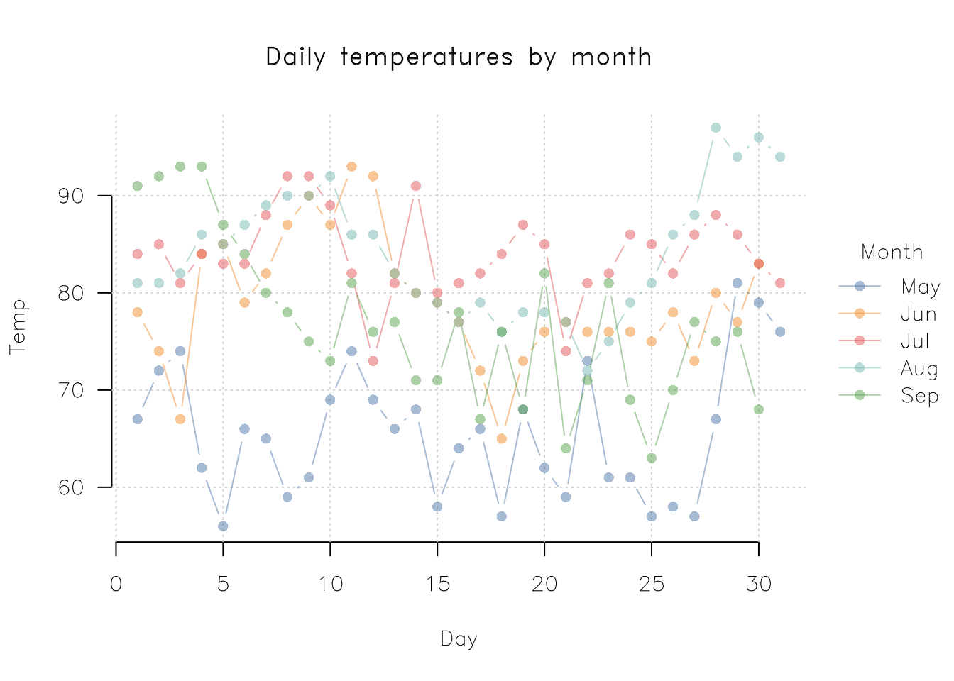
a numeric in the range [0,1] for adjusting the alpha channel of the color palette, where 0 means transparent and 1 means opaque. Use fractional values, e.g. 0.5 for semi-transparency.
|
cex
|
character expansion. A numerical vector (can be a single value) giving the amount by which plotting characters and symbols should be scaled relative to the default. Note that NULL is equivalent to 1.0, while NA renders the characters invisible. There are two additional considerations, specifically for points-alike plot types (e.g. “p”):
-
users can also supply a special cex = “by” convenience argument, in which case the character expansion will automatically adjust by group too. The range of this character expansion is controlled by the clim argument in the respective types; see type_points() for example.
-
passing a cex vector of equal length to the main x and y variables (e.g., another column in the same dataset) will yield a "bubble"plot with its own dedicated legend. This can provide a useful way to visualize an extra dimension of the data; see Examples.
|
add
|
logical. If TRUE, then elements are added to the current plot rather than drawing a new plot window. Note that the automatic legend for the added elements will be turned off. See also tinyplot_add, which provides a convenient wrapper around this functionality for layering on top of an existing plot without having to repeat arguments.
|
draw
|
a function that draws directly on the plot canvas (before x and y are plotted). The draw argument is primarily useful for adding common elements to each facet of a faceted plot, e.g. abline or text. Note that this argument is somewhat experimental and that no internal checking is done for correctness; the provided argument is simply captured and evaluated as-is within tinyplot() and thus has access to the local definition of all variables such as x, y, etc. See Examples.
|
empty
|
logical indicating whether the interior plot region should be left empty. The default is FALSE. Setting to TRUE has a similar effect to invoking type = “n” above, except that any legend artifacts owing to a particular plot type (e.g., lines for type = “l” or squares for type = “area”) will still be drawn correctly alongside the empty plot. In contrast,type = “n” implicitly assumes a scatterplot and so any legend will only depict points.
|
restore.par
|
a logical value indicating whether the par settings prior to calling tinyplot should be restored on exit. Defaults to FALSE, which makes it possible to add elements to the plot after it has been drawn. However, note the the outer margins of the graphics device may have been altered to make space for the tinyplot legend. Users can opt out of this persistent behaviour by setting to TRUE instead. See also get_saved_par for another option to recover the original par settings, as well as longer discussion about the trade-offs involved.
|
file
|
character string giving the file path for writing a plot to disk. If specified, the plot will not be displayed interactively, but rather sent to the appropriate external graphics device (i.e., png, jpeg, pdf, or svg). As a point of convenience, note that any global parameters held in (t)par are automatically carried over to the external device and don’t need to be reset (in contrast to the conventional base R approach that requires manually opening and closing the device). The device type is determined by the file extension at the end of the provided path, and must be one of ".png", ".jpg" (".jpeg"), ".pdf", or ".svg". (Other file types may be supported in the future.) The file dimensions can be controlled by the corresponding width and height arguments below, otherwise will fall back to the “file.width” and “file.height” values held in tpar (i.e., both defaulting to 7 inches, and where the default resolution for bitmap files is also specified as 300 DPI).
|
width
|
numeric giving the plot width in inches. Together with height, typically used in conjunction with the file argument above, overriding the default values held in tpar(“file.width”, “file.height”). If either width or height is specified, but a corresponding file argument is not provided as well, then a new interactive graphics device dimensions will be opened along the given dimensions. Note that this interactive resizing may not work consistently from within an IDE like RStudio that has an integrated graphics windows.
|
height
|
numeric giving the plot height in inches. Same considerations as width (above) apply, e.g. will default to tpar(“file.height”) if not specified.
|
asp
|
the y/xy/x aspect ratio, see plot.window.
|
theme
|
keyword string (e.g. “clean”) or list defining a theme. Passed on to tinytheme, but reset upon exit so that the theme effect is only temporary. Useful for invoking ephemeral themes.
|
formula
|
a formula that optionally includes grouping variable(s) after a vertical bar, e.g. y ~ x | z. One-sided formulae are also permitted, e.g. ~ y | z. Only a single y and x variable (if any) must be specified but multiple grouping variables can be included in different ways, e.g. y ~ x | z1:z2 or y ~ x | z1 + z2. (These two representations are treated as equivalent; both are parsed as interaction(z1, z2) internally.) If arithmetic operators are used for transforming variables, they should be wrapped in I(), e.g., I(y1/y2) ~ x. Note that the formula and x arguments should not be specified in the same call.
|
subset, na.action, drop.unused.levels
|
arguments passed to model.frame when extracting the data from formula and data.
|