Lightweight extension of the base R graphics system

userR! 2025
August 9, 2025
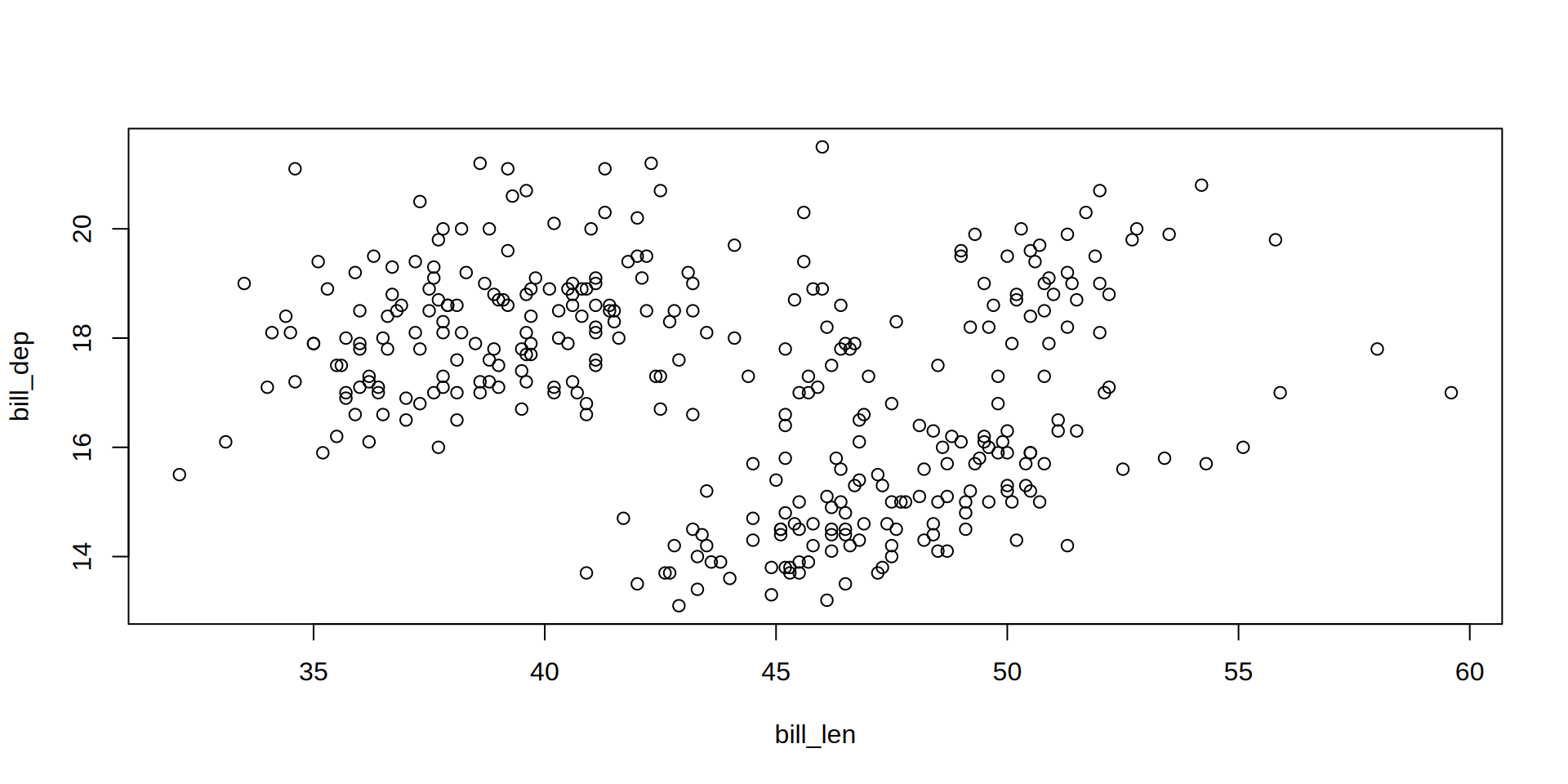
base::plot
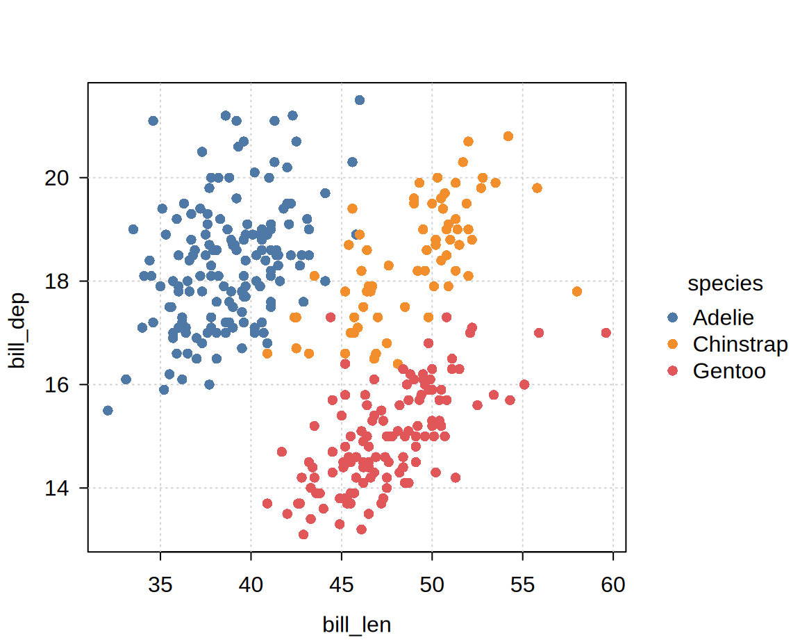
Simple scatter plot
base::plot
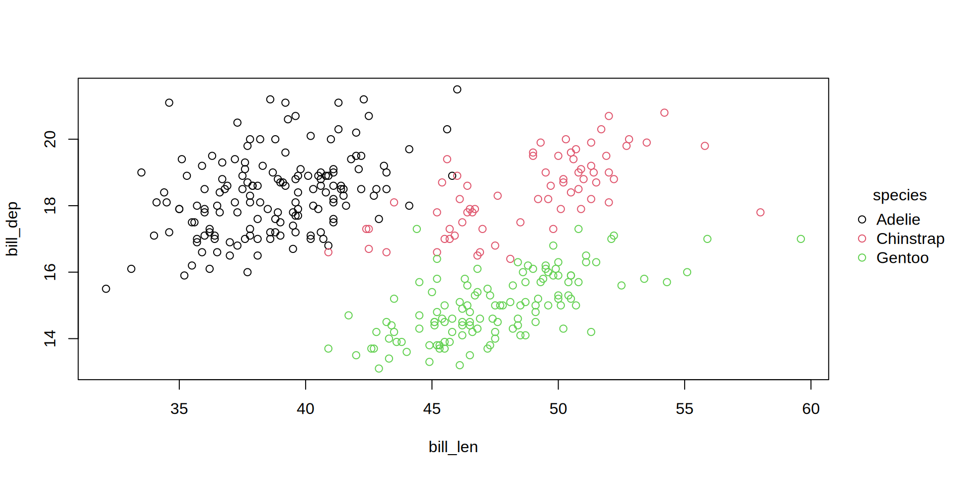
Let’s add some grouping
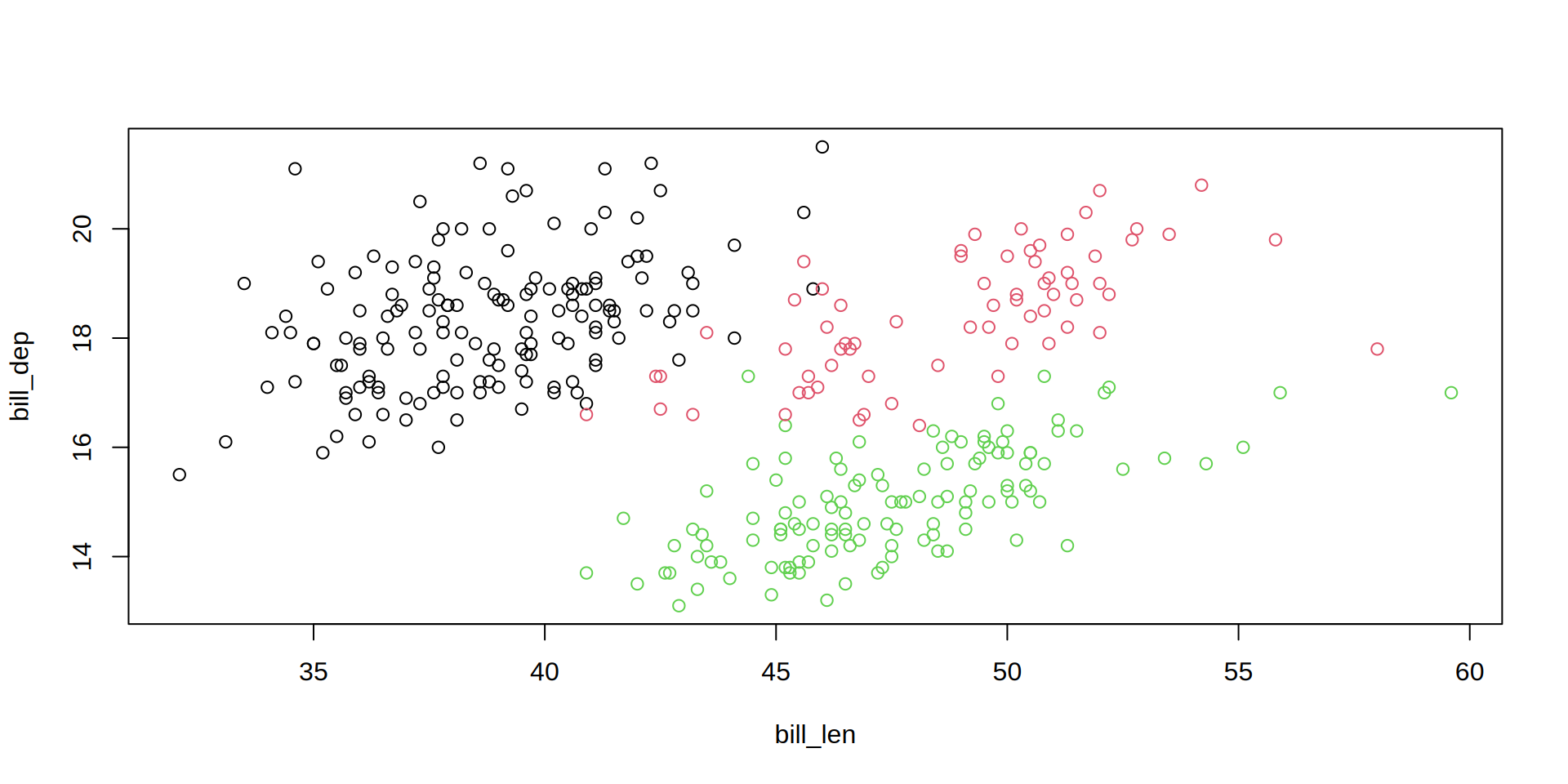
NB: col = species works here because species is a factor.
base::plot
Add a legend

Q: Can you spot the error?
base::plot
Add a legend
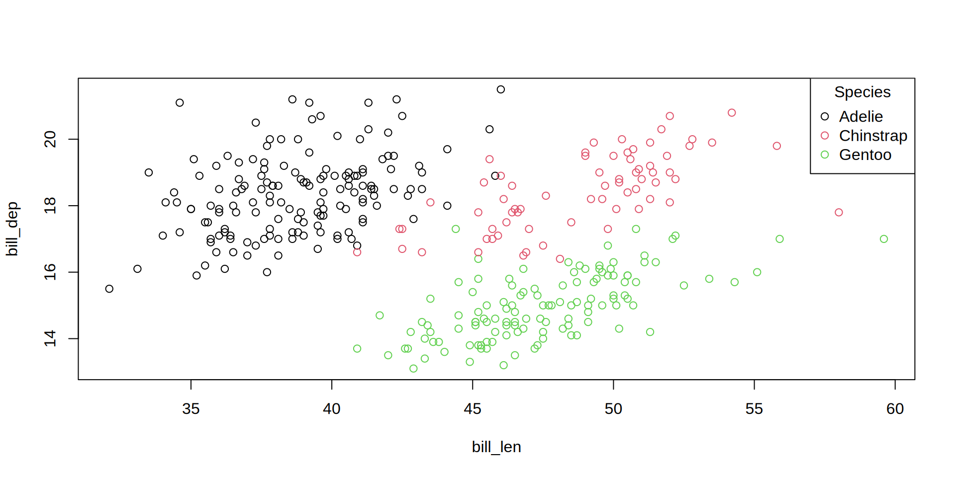
A: We should have used levels(species), not unique(species).
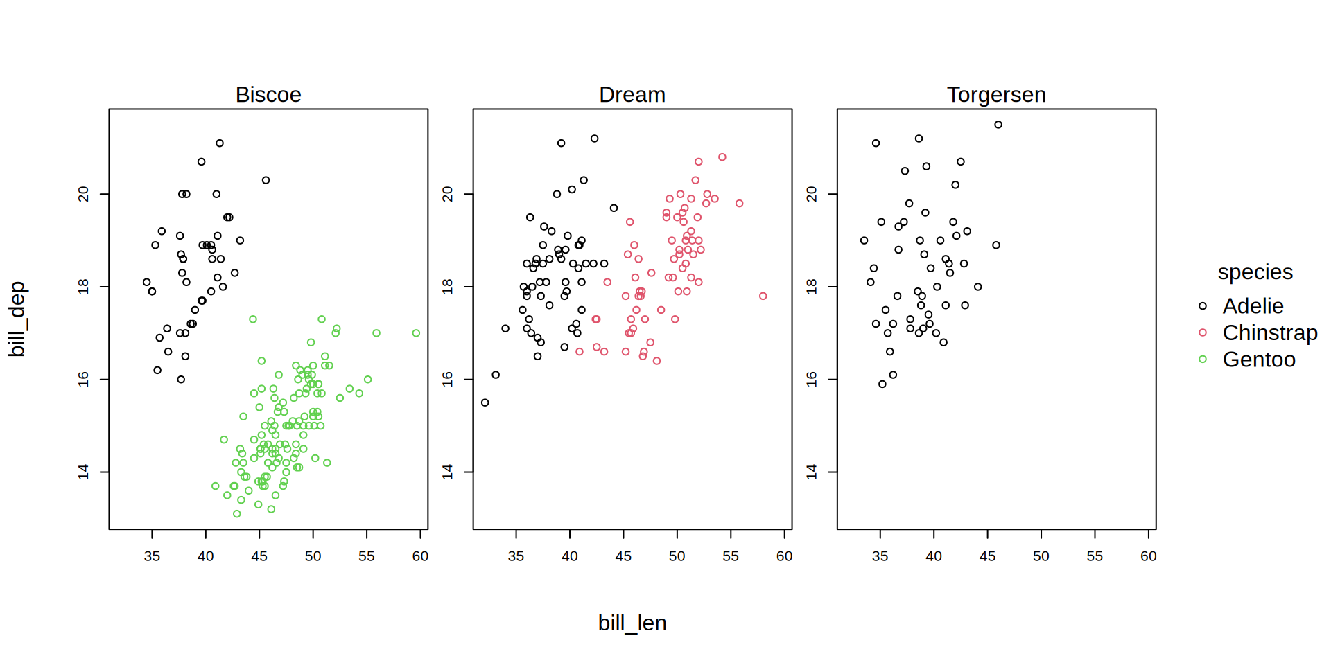
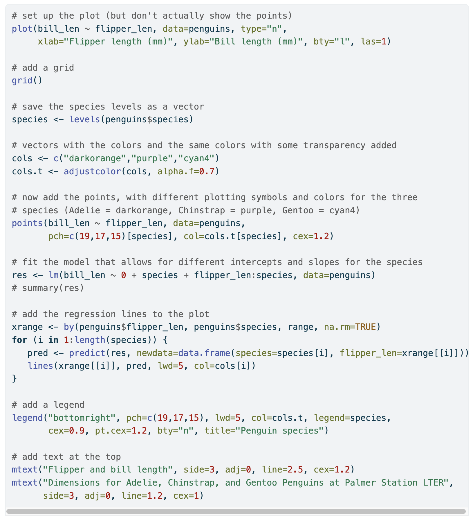
base::plot
How about a different plot type?
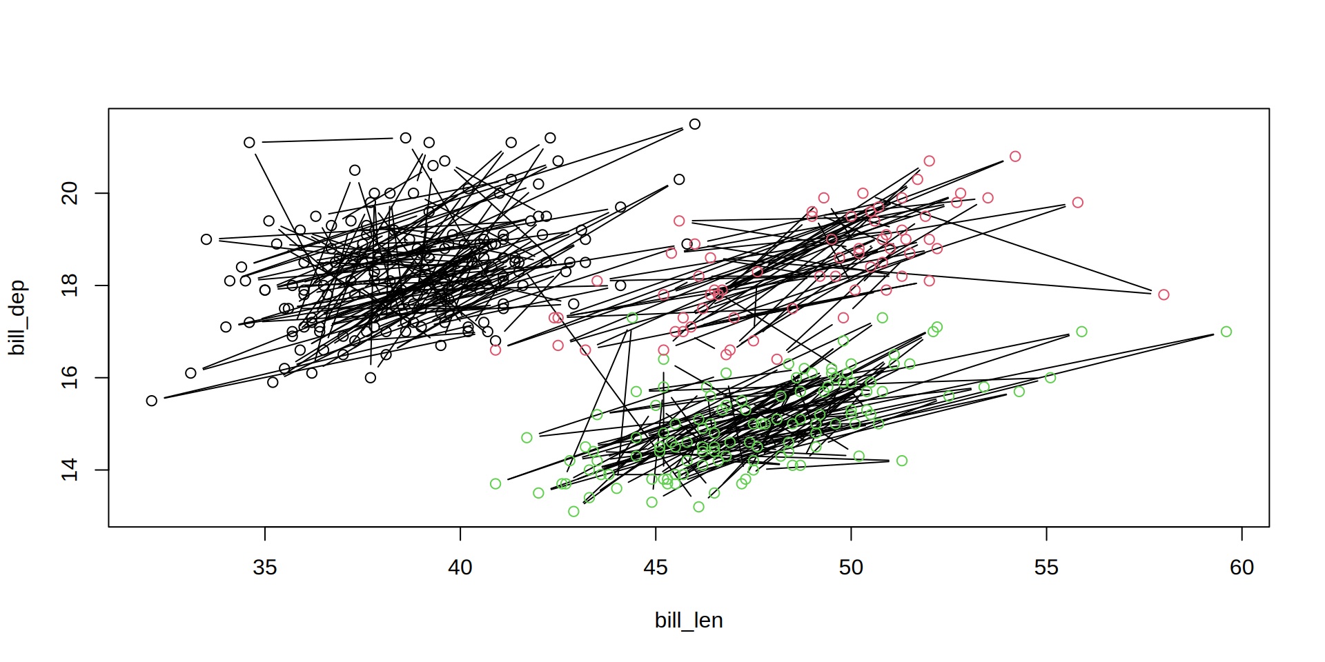
Ugh… our grouped coloring logic only works for the “points” components.
Enter tinyplot
![]()
Tip
In the plots that follow, plt(...) is a shorthand alias for tinyplot(...).
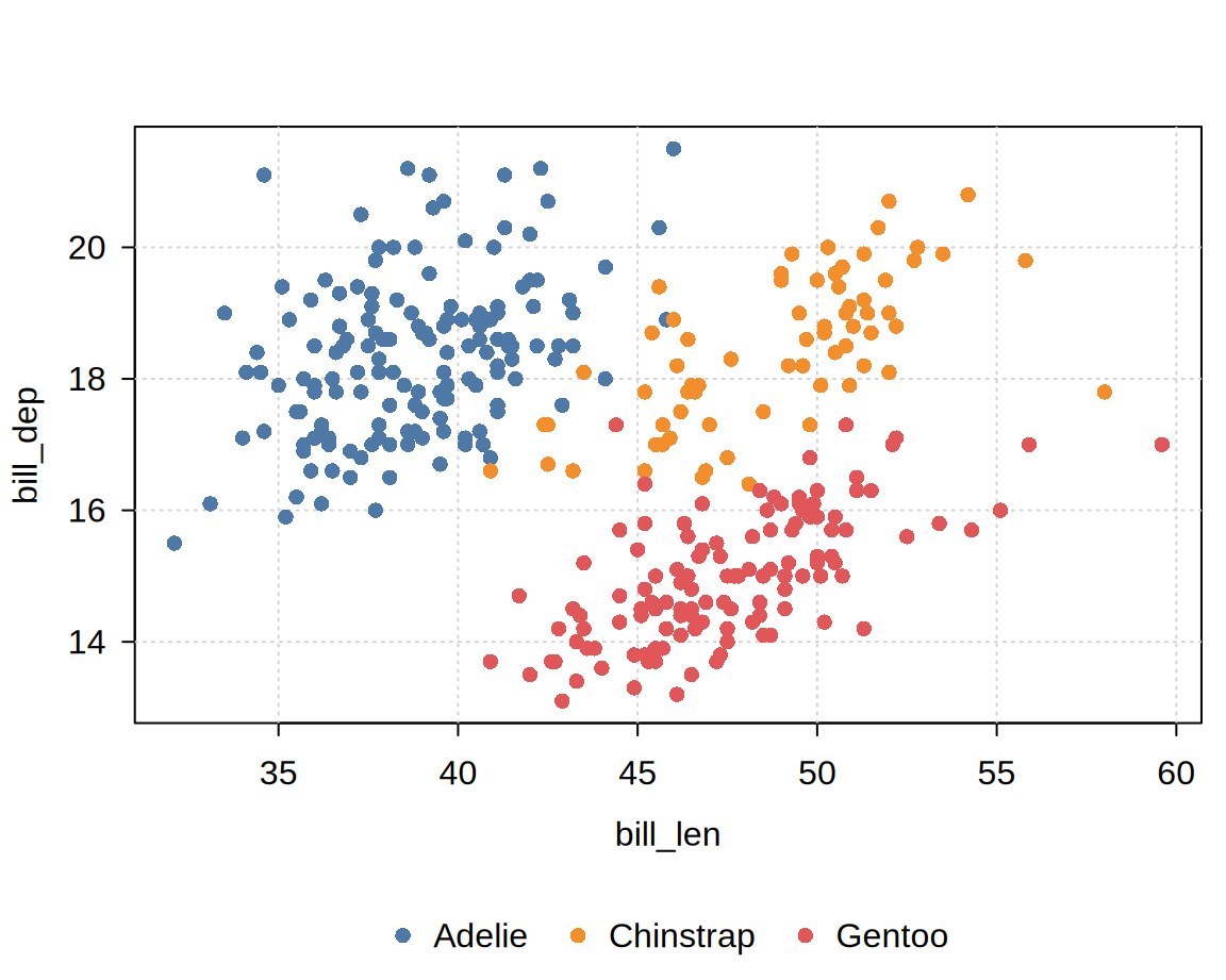
tinyplot::plt
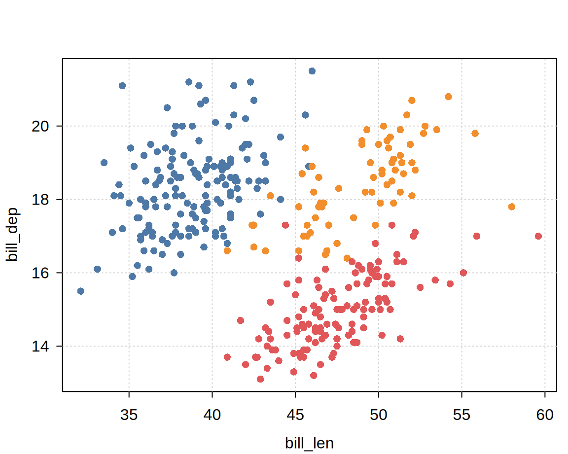
Simplest case: drop-in replacement for base::plot

But we can do a lot more than that…
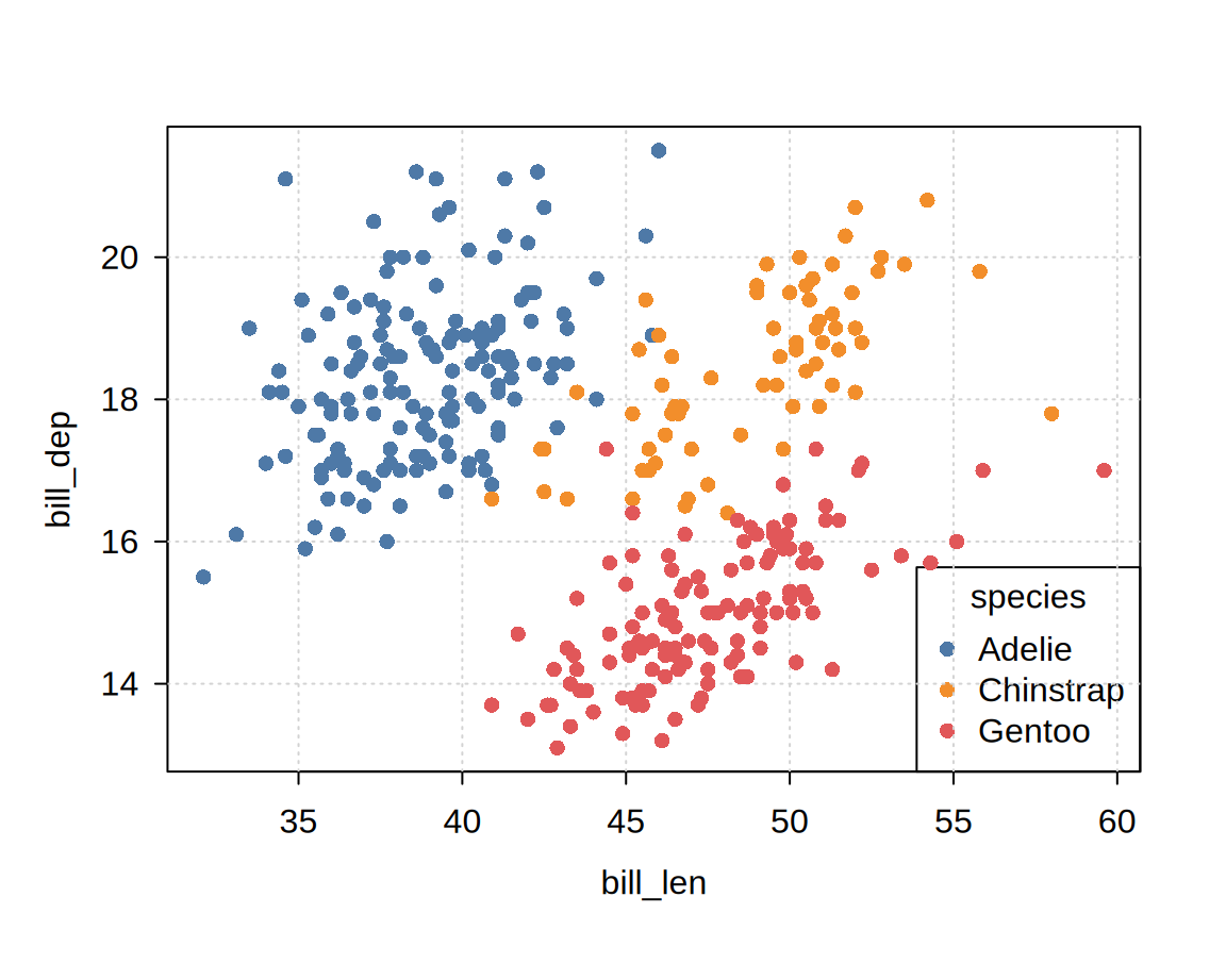
tinyplot::plt
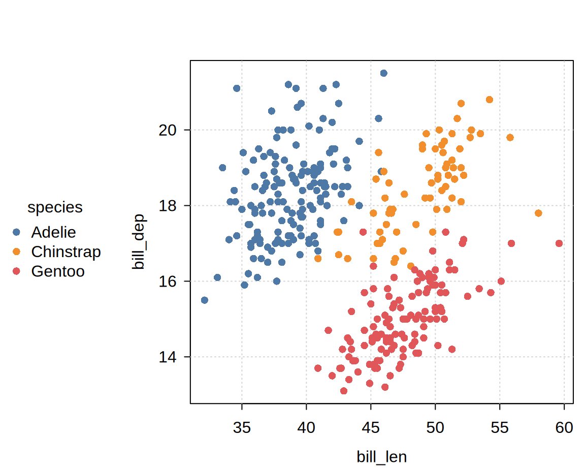
How do we automate the legend mapping?
tinyplot::plt
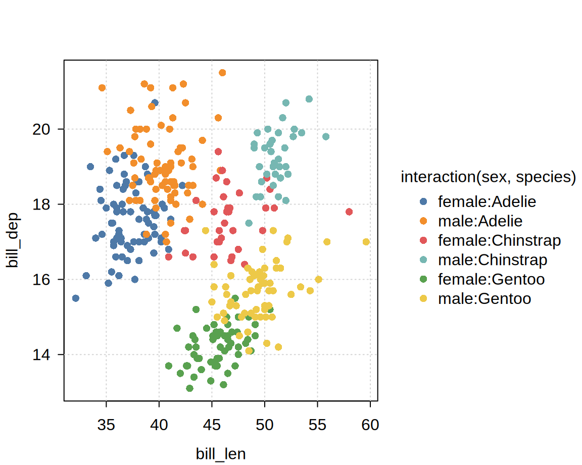
How do we group by additional variables?
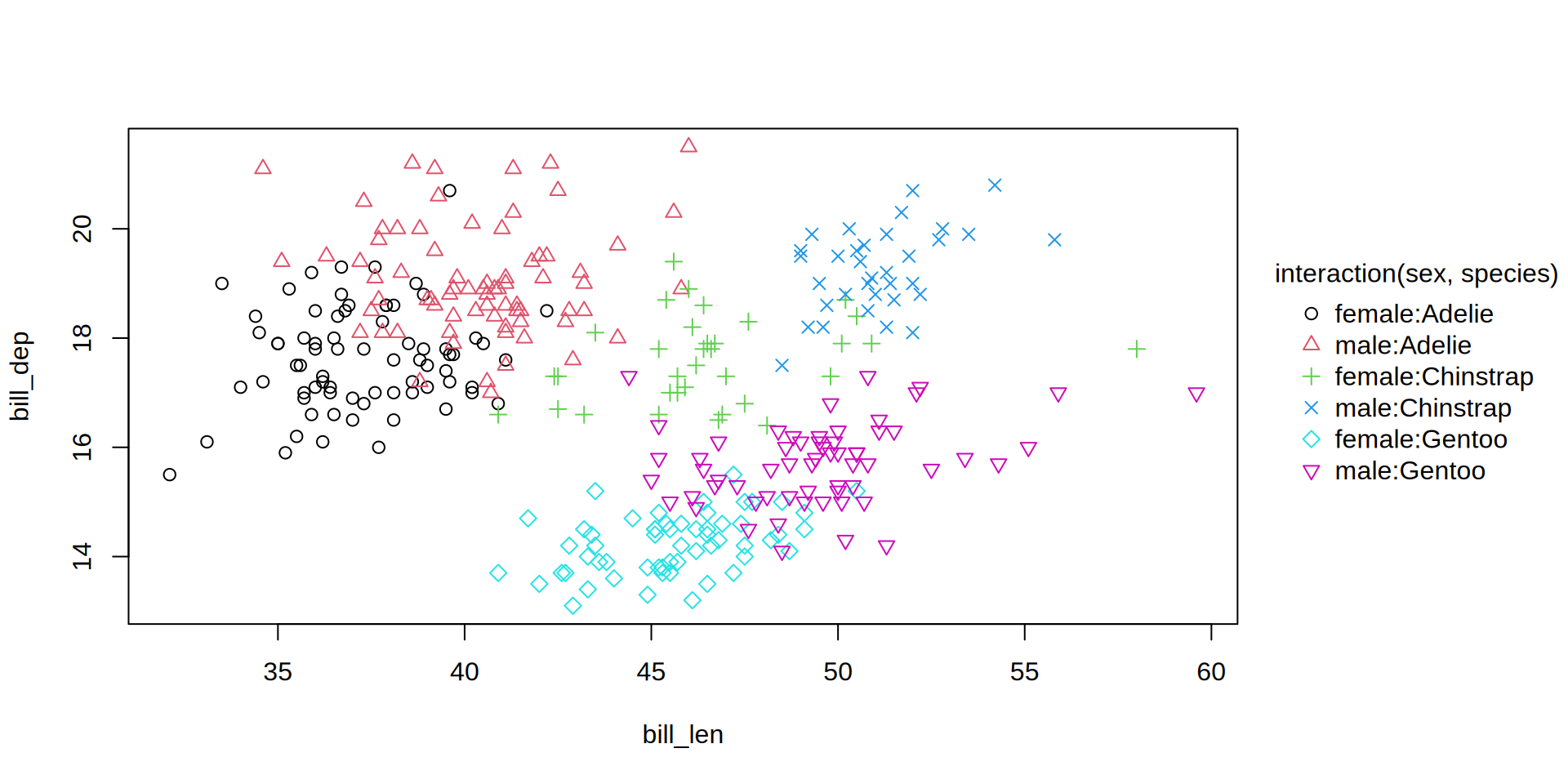
tinyplot::plt
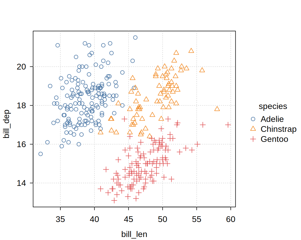
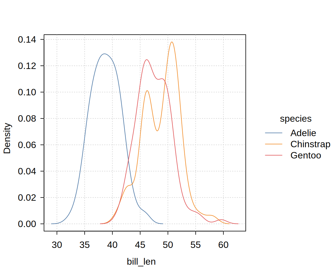
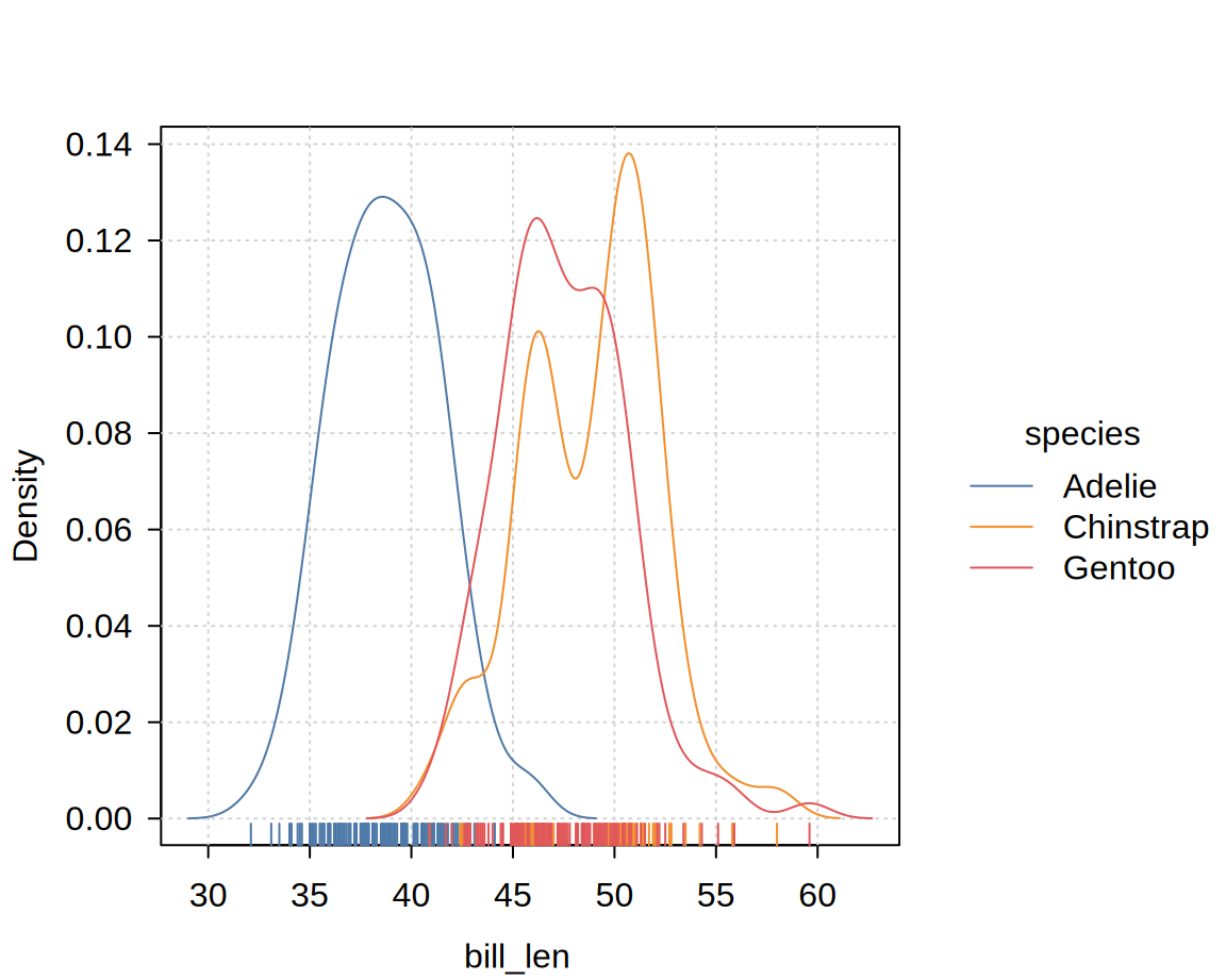
What if we want groups with a different plot type?
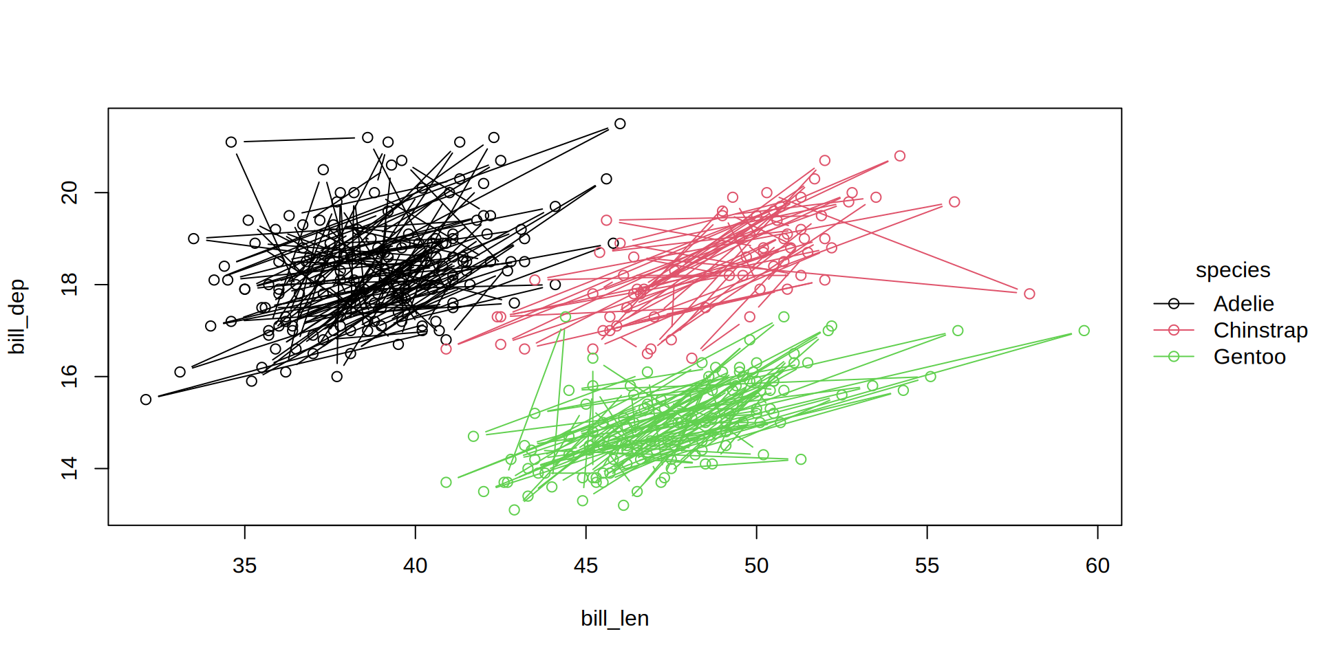
tinyplot::plt
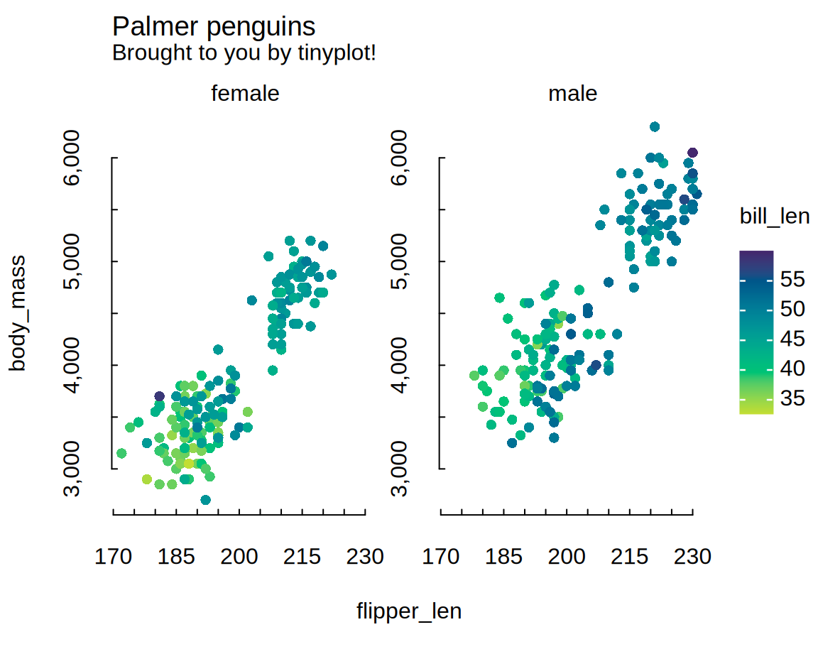
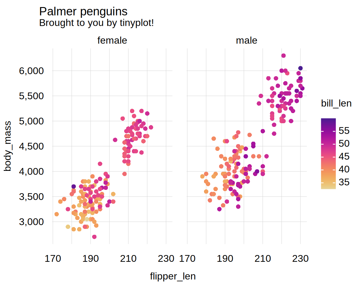
What if we need to group by a continuous variable?
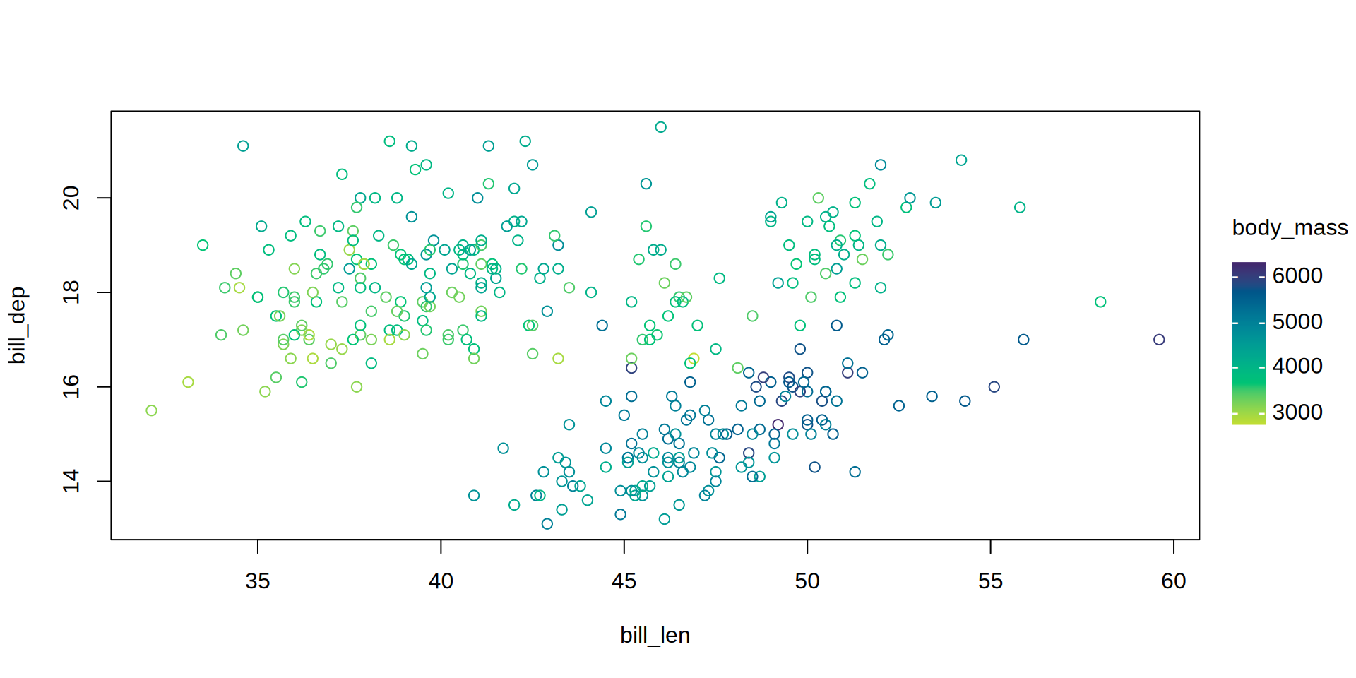
tinyplot::plt
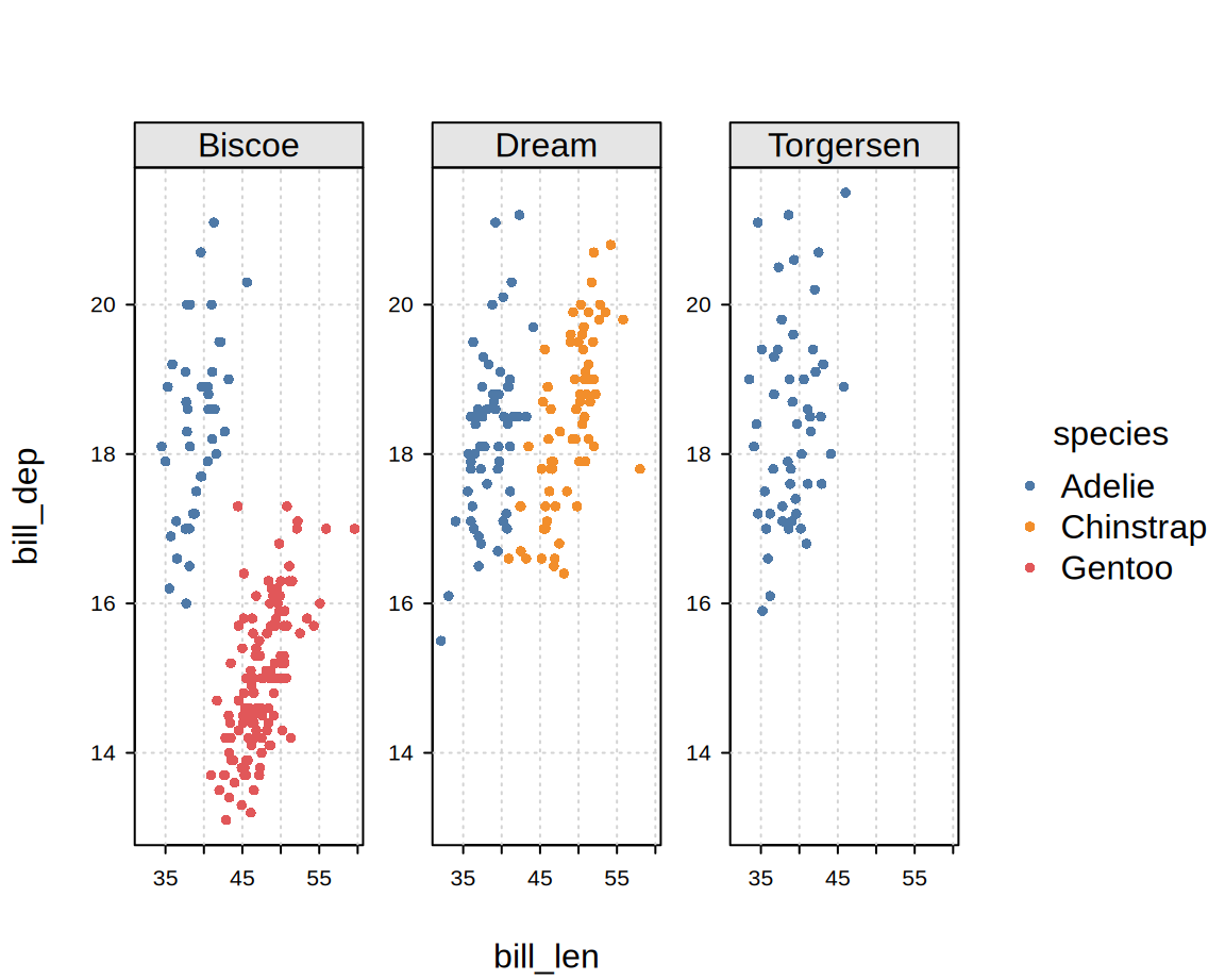
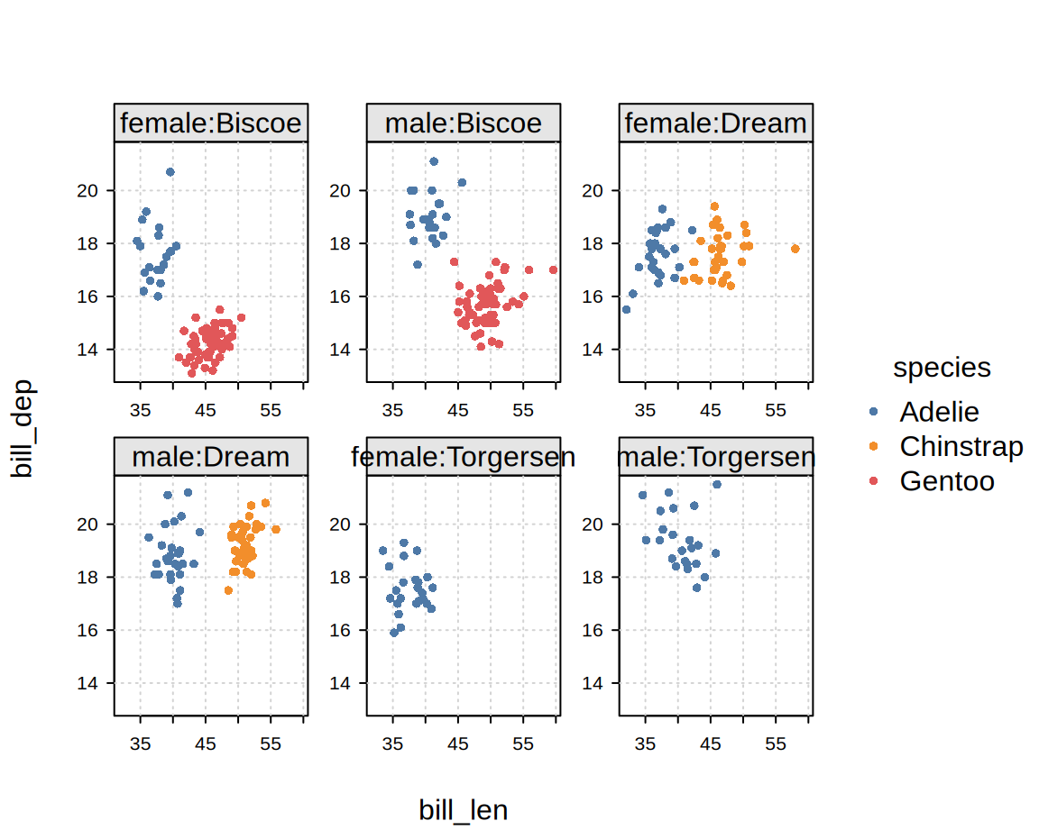
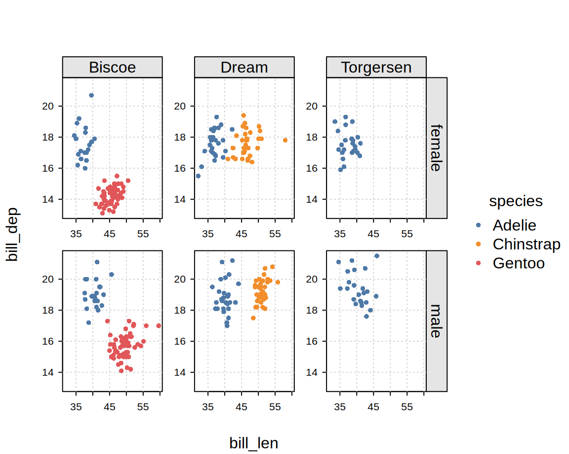
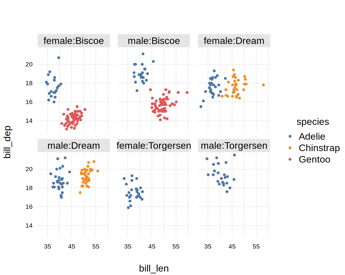
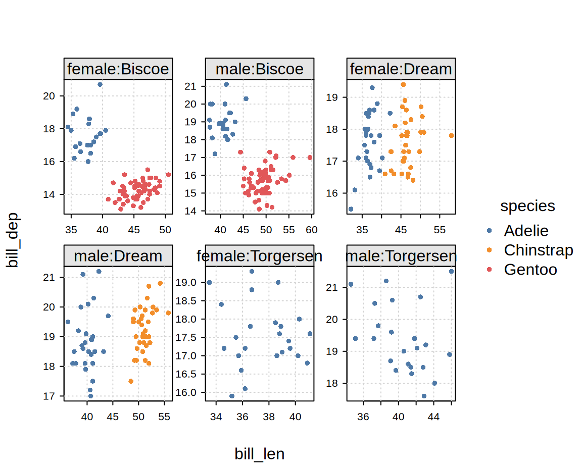
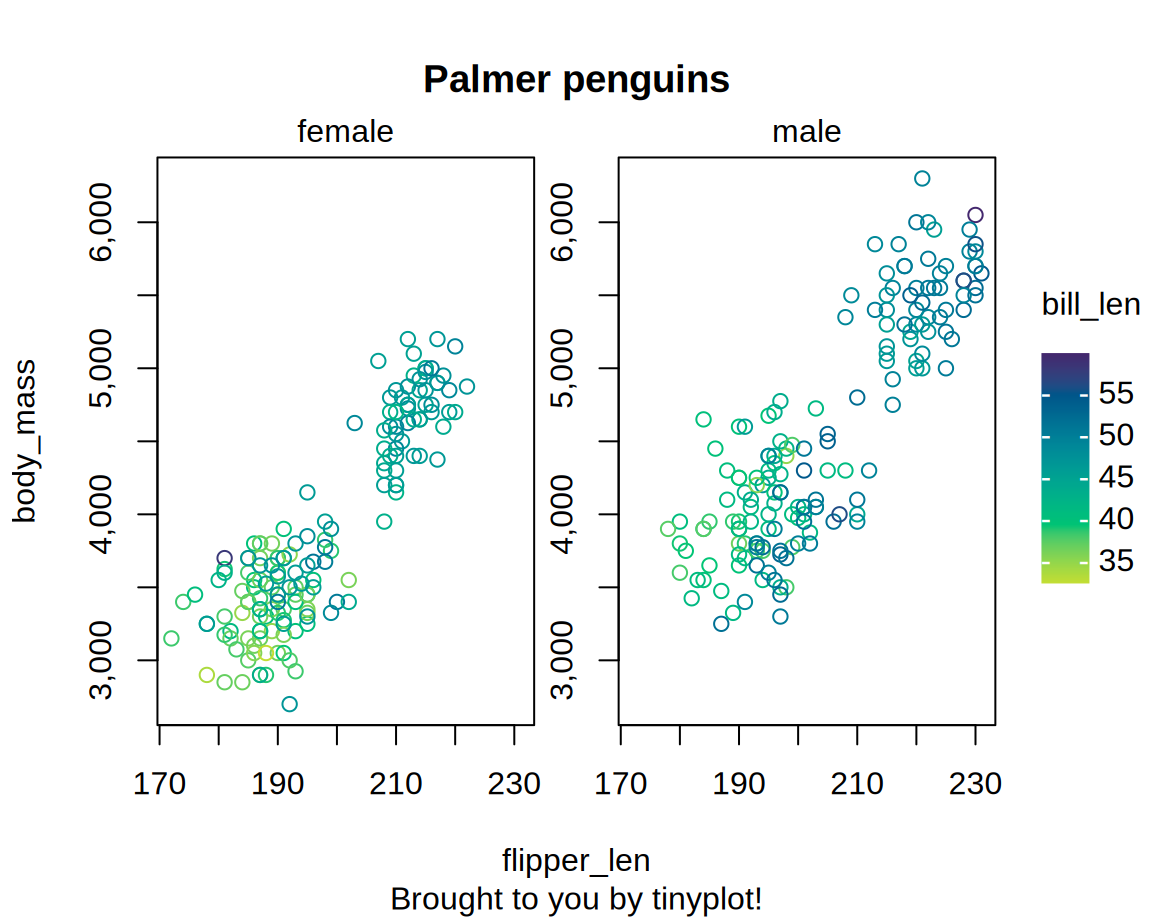
What if we need to facet by another variable?
tinyplot::plt
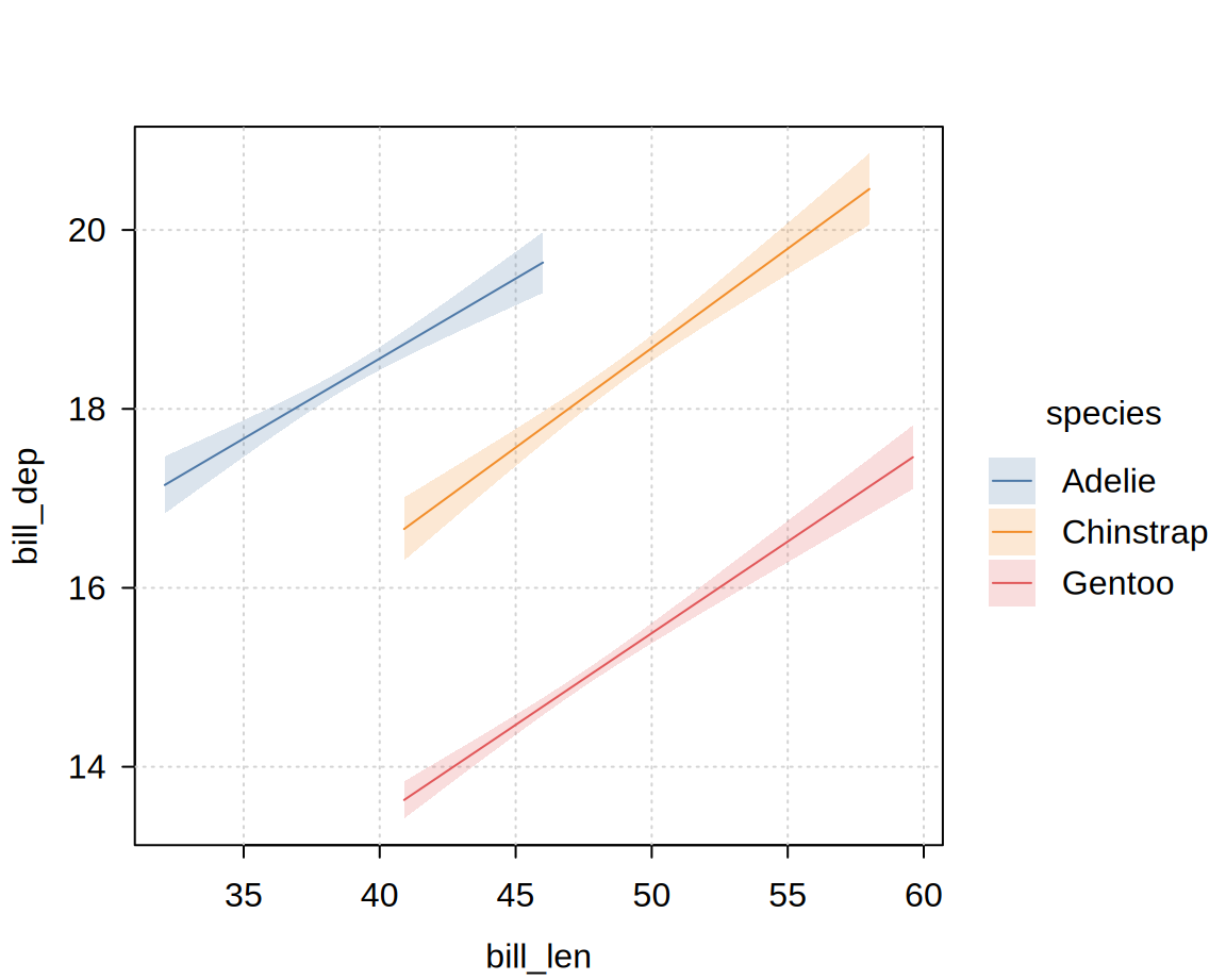
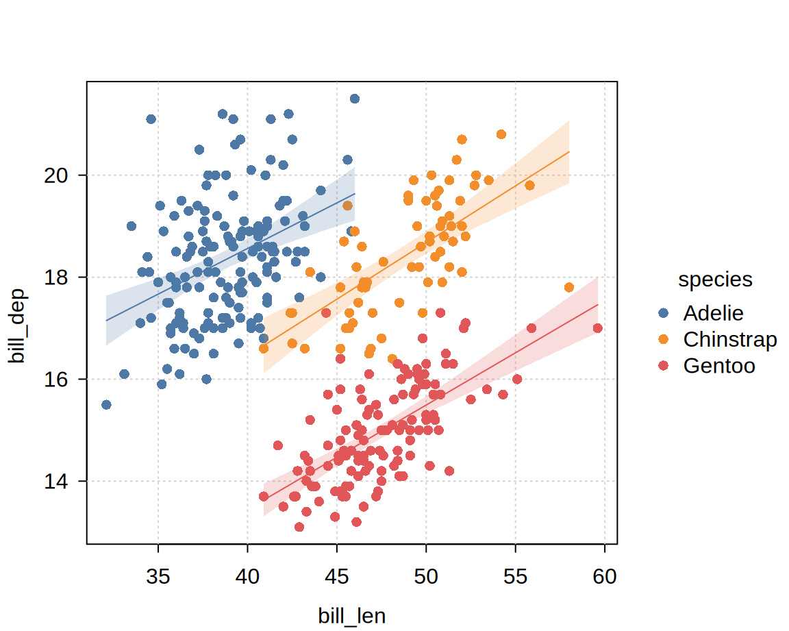
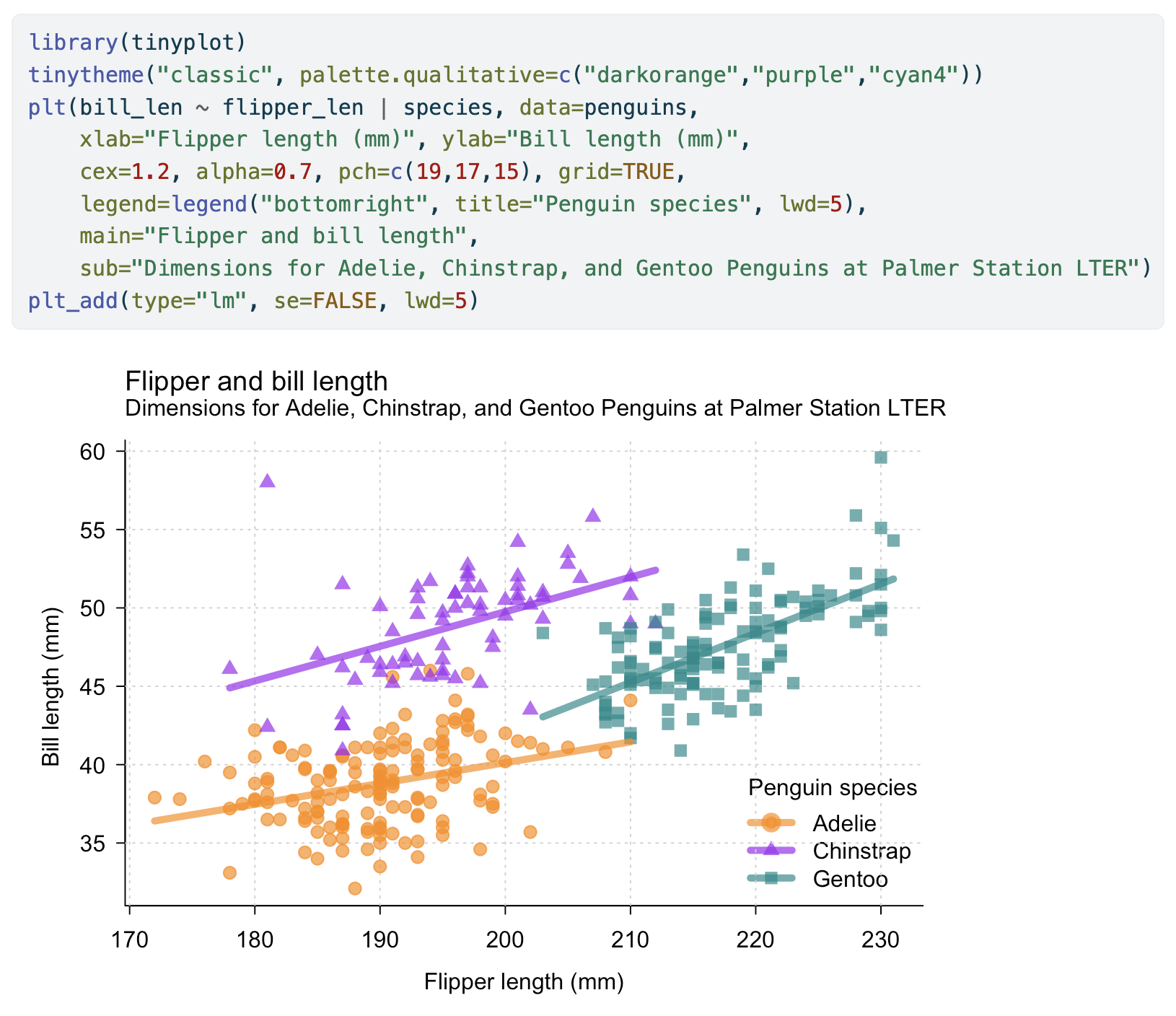
What if we want to add a summary function, e.g. regression fit?
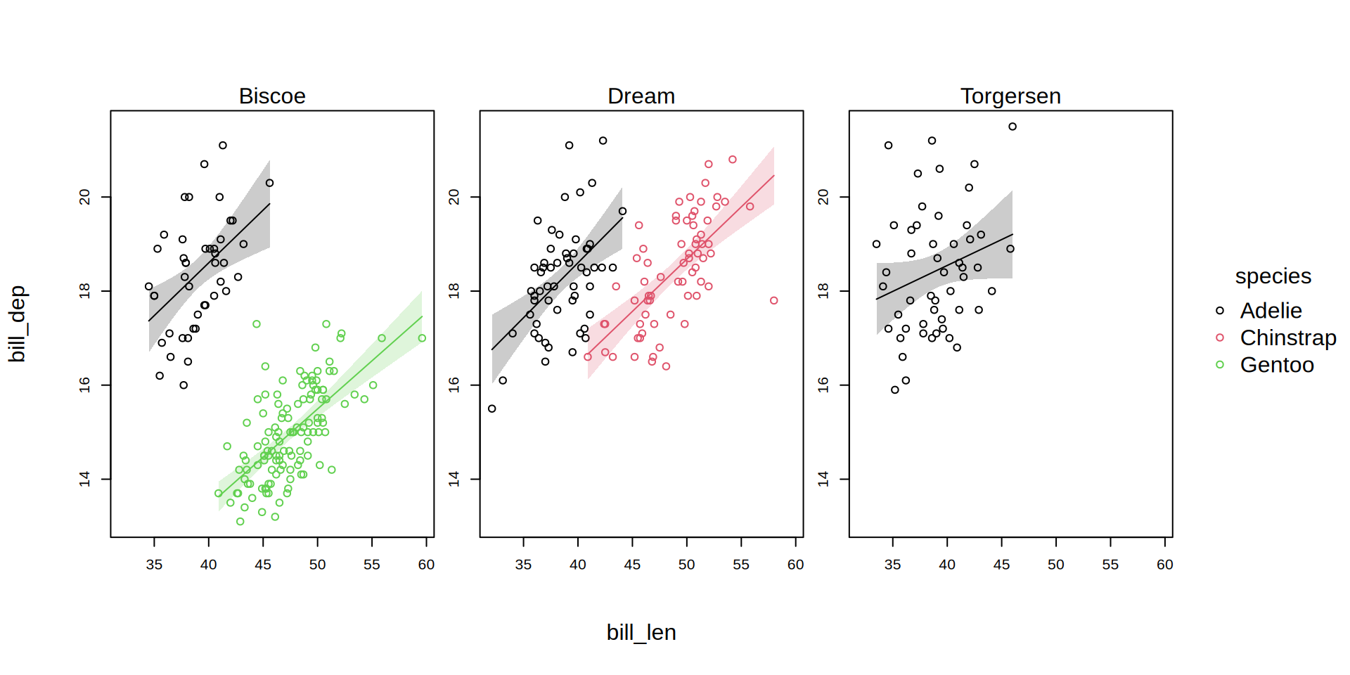
tinyplot::plt
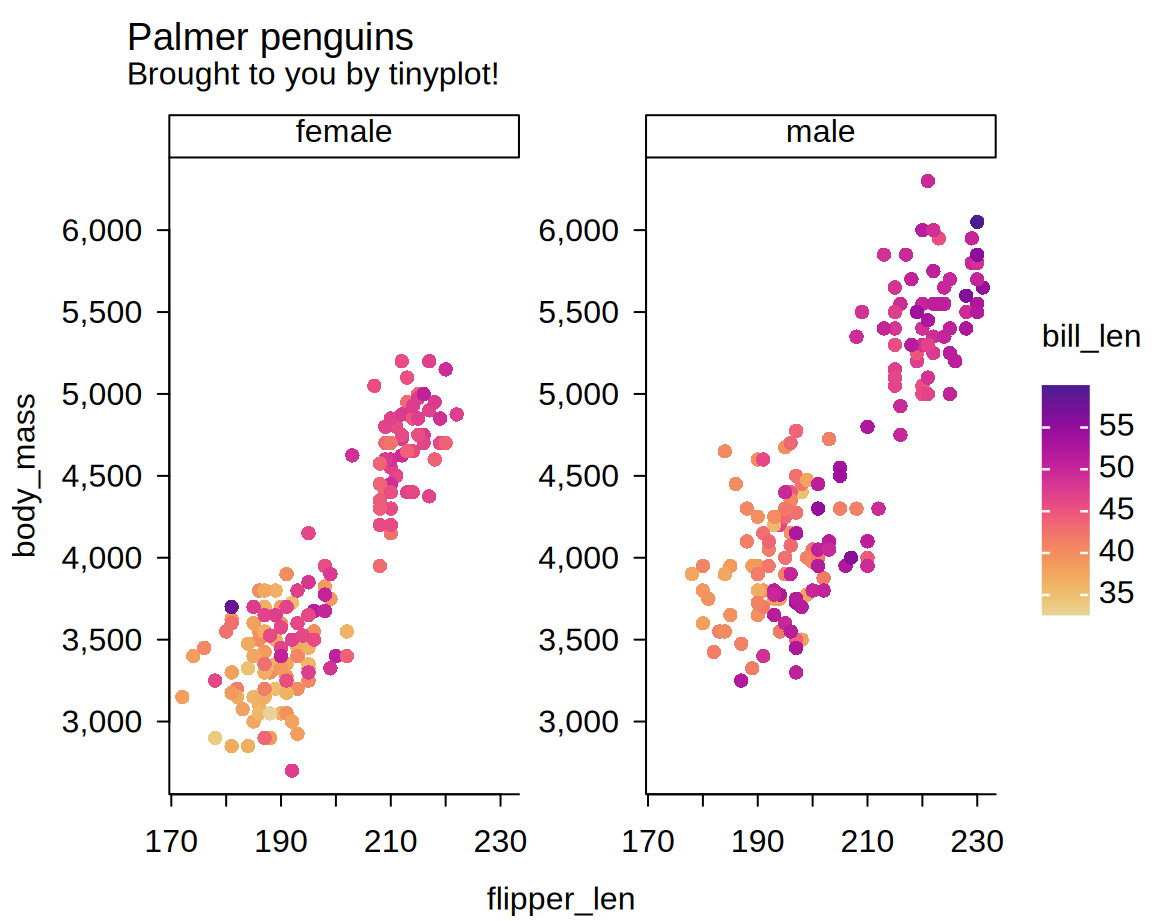
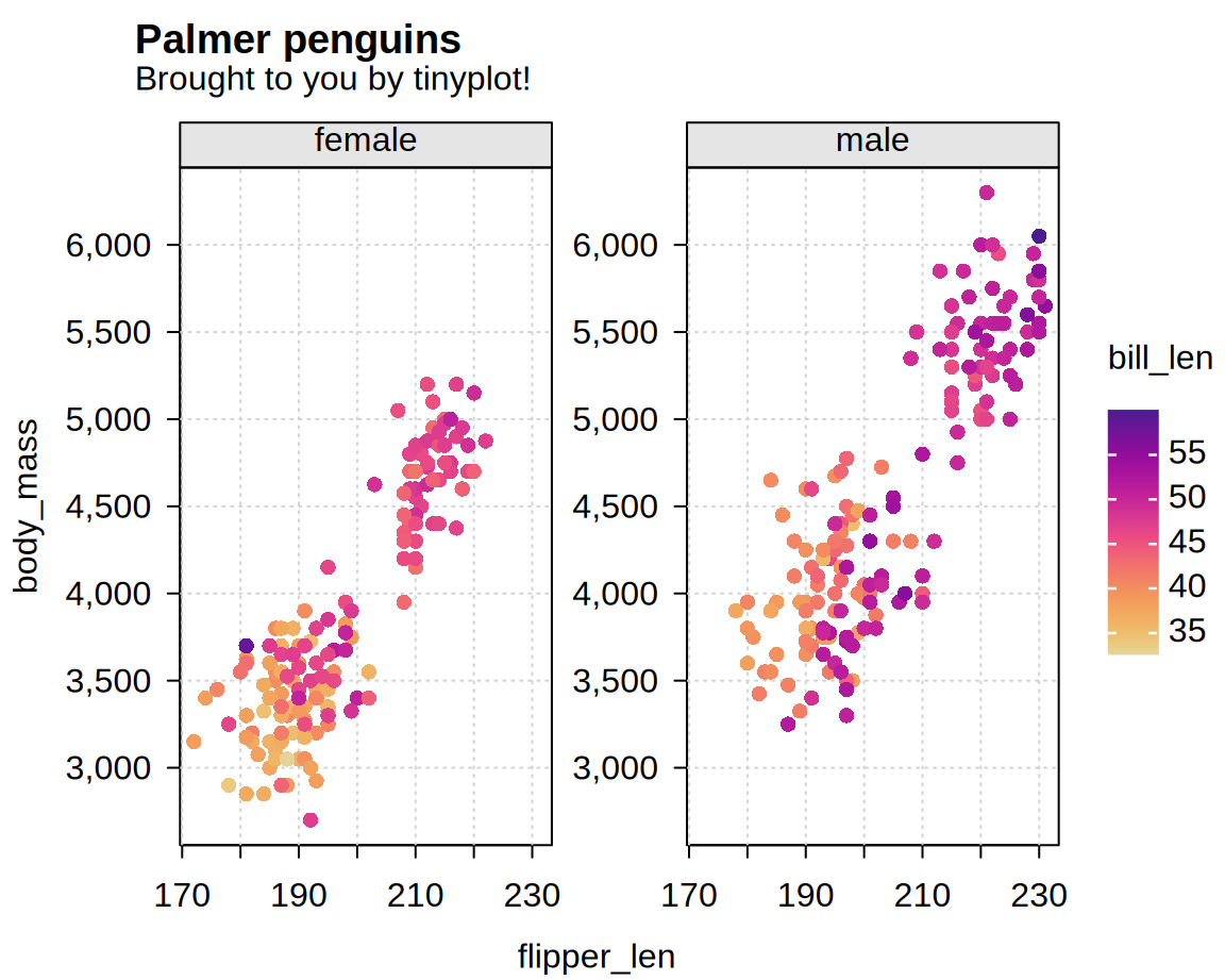
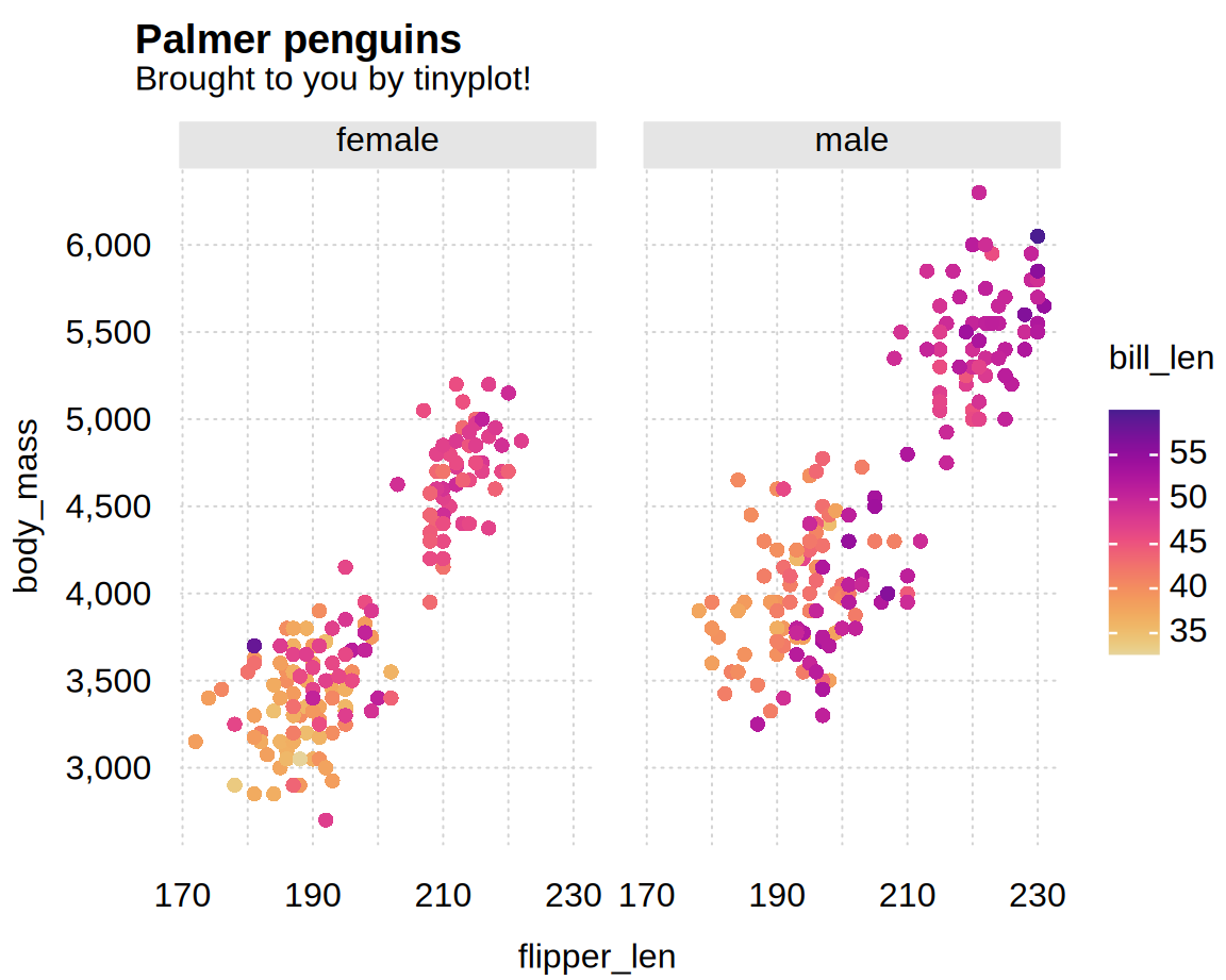
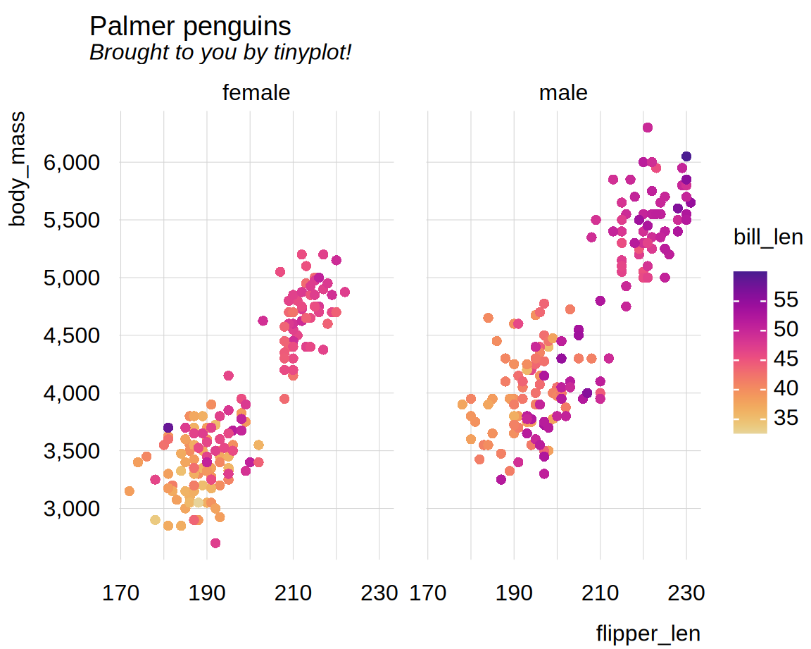
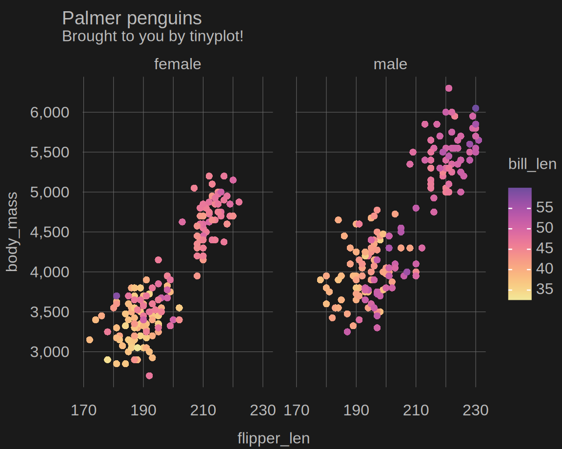
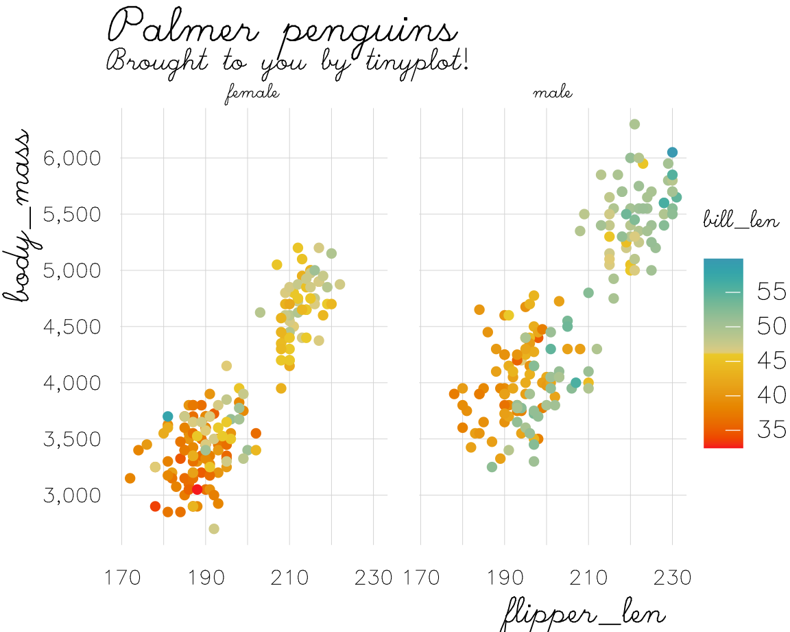
The plots are kind of ugly. Can we make them look better?
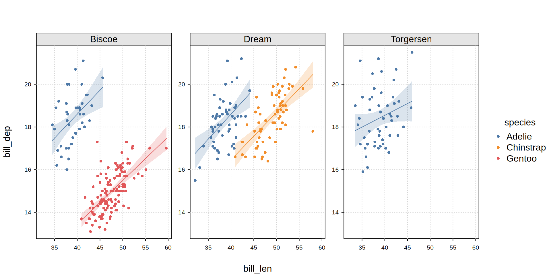
NB: Themes are persistent; subsequent (tiny)plots will inherit this aesthetic.
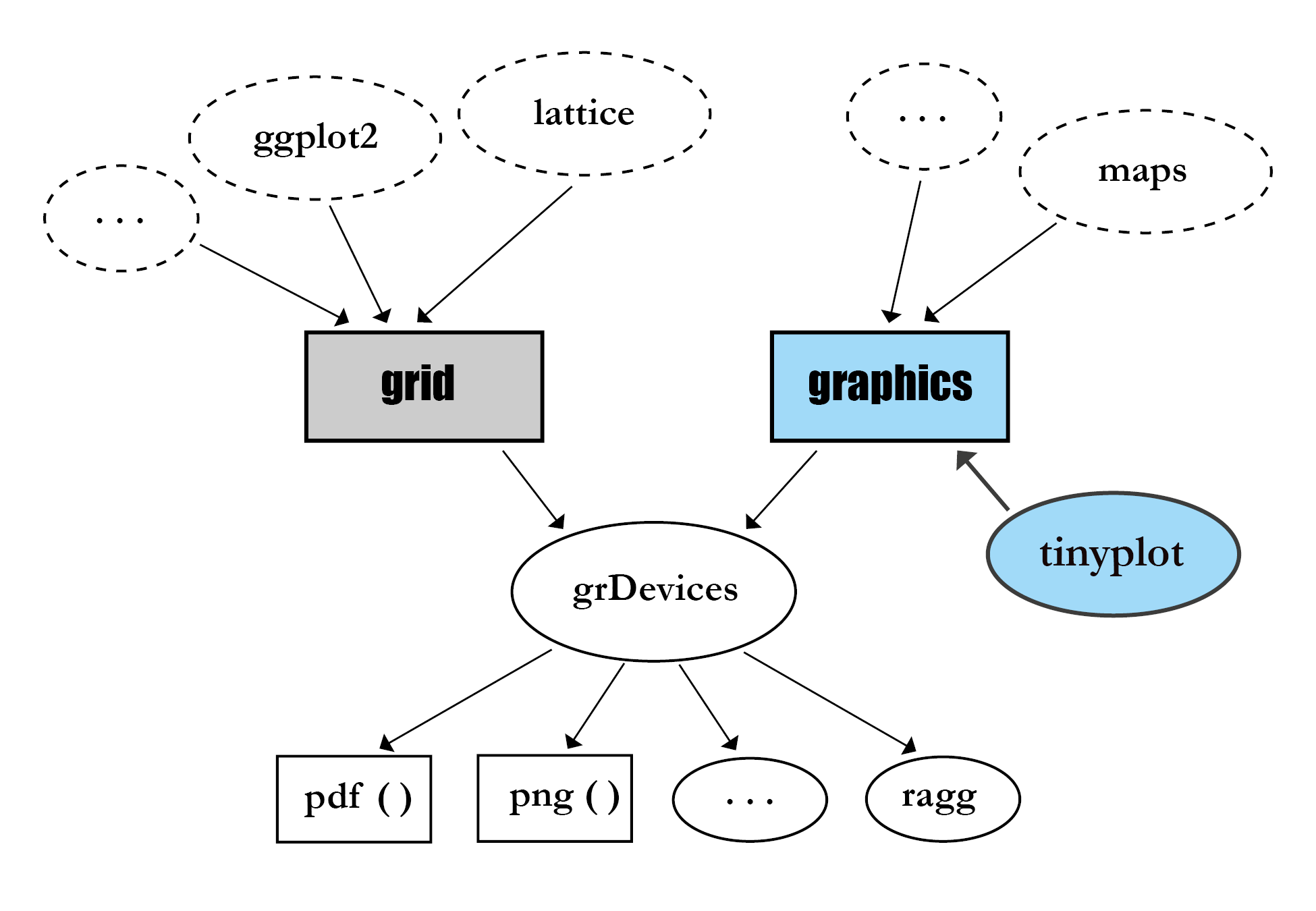
grid vs graphics
R has two low-level graphics systems
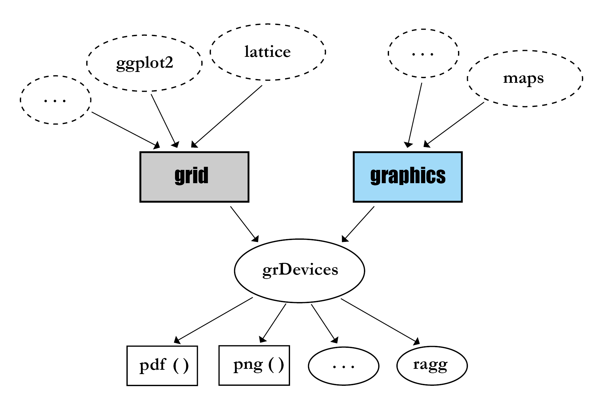
Note: Adapted from Murrell (2023).
Base graphics in R
Very flexible… but tricksy
Base graphics can produce amazing plots.
plot()is just an (opinionated) wrapper around lower-level functions. (Koncevičius 2022)
- This is very powerful in expert hands. (Mayakonda 2022)
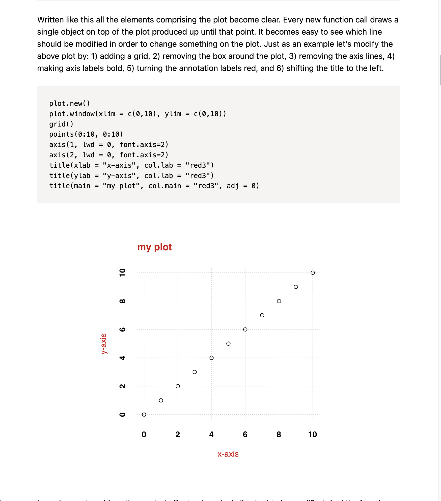
But going beyond the defaults is often (much) more work that I want to do.
grid vs graphics (redux)
R has two low-level graphics systems
grid vs graphics (redux)
R has two low-level graphics systems
grid vs graphics (redux)
R has two low-level graphics systems
tinyplot goals:
- Make base R graphics more user-friendly.
- Improved feature parity vs. grid-based 📦s like ggplot2 and lattice.
Origin story 🤝
Collaboration
A basic version of the core routine (then called “plot2.R”) sat on my computer for a long time.
I eventually packaged it up… and invited two key collaborators:


tinyplot API
Group(s) after the pipe |
tinyplot API
Groups map to colors; use the "by" keyword for other mappings
Also works for lwd, lty, etc.
tinyplot API
Legend can be moved, customized and turned off
A "!" suffix places the legend outside the plot area.
tinyplot API
facets
tinyplot API
types
tinyplot API
Layers
tinyplot API
Themes
Quickfire gallery
histogram
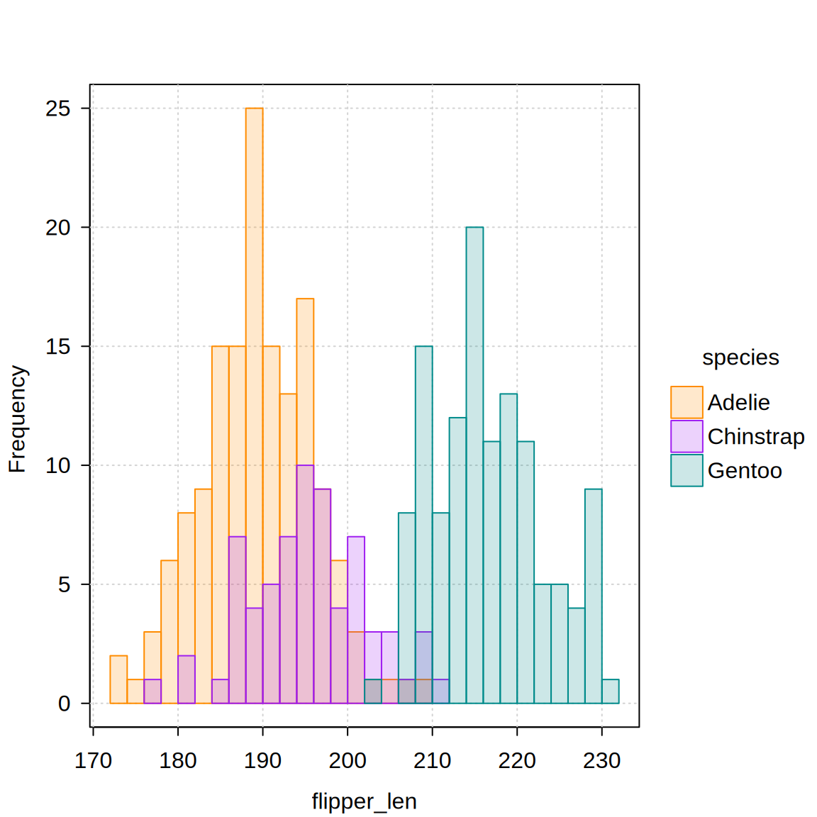
Quickfire gallery
box plots
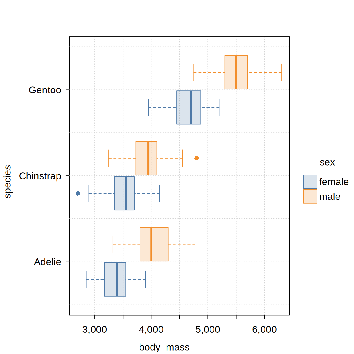
Quickfire gallery
violin plots
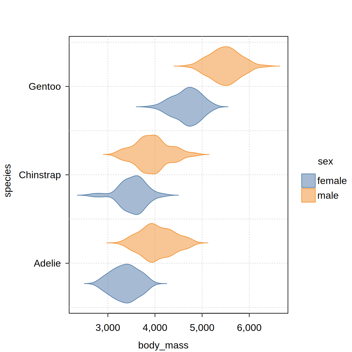
Quickfire gallery
error bars
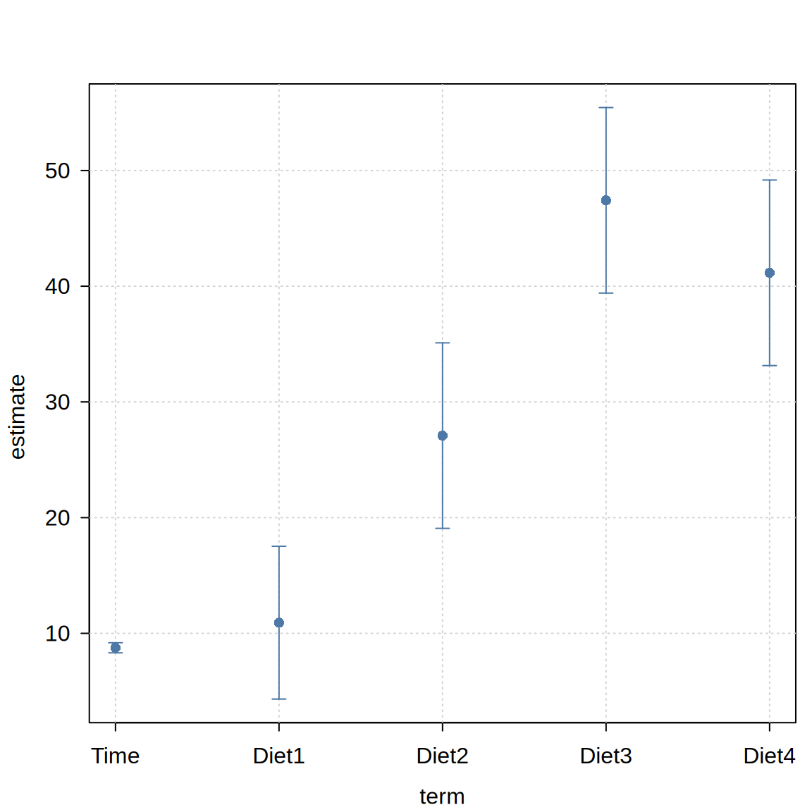
Quickfire gallery
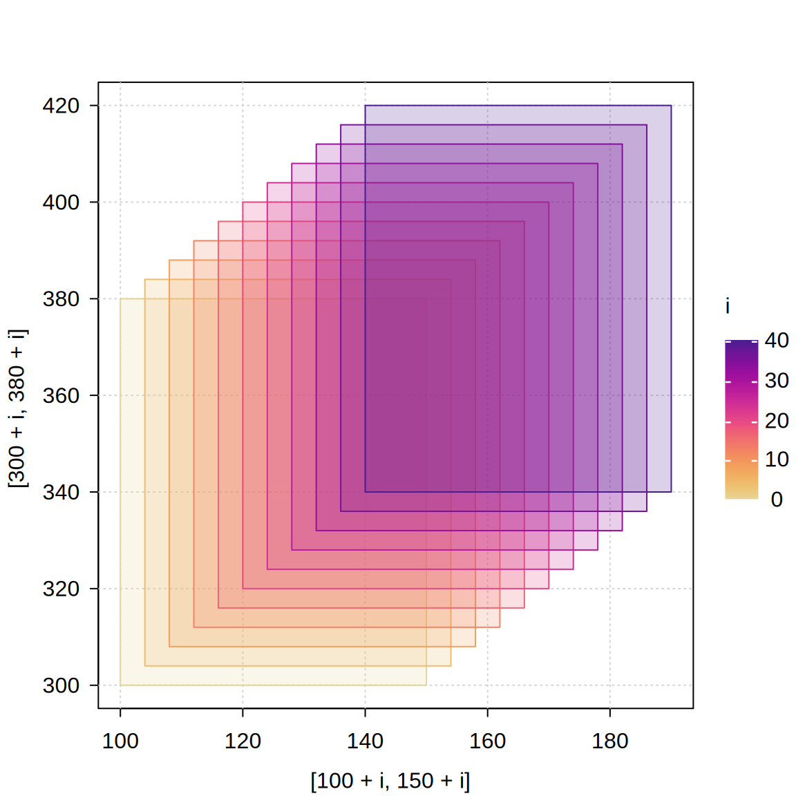
rectangles
Quickfire gallery
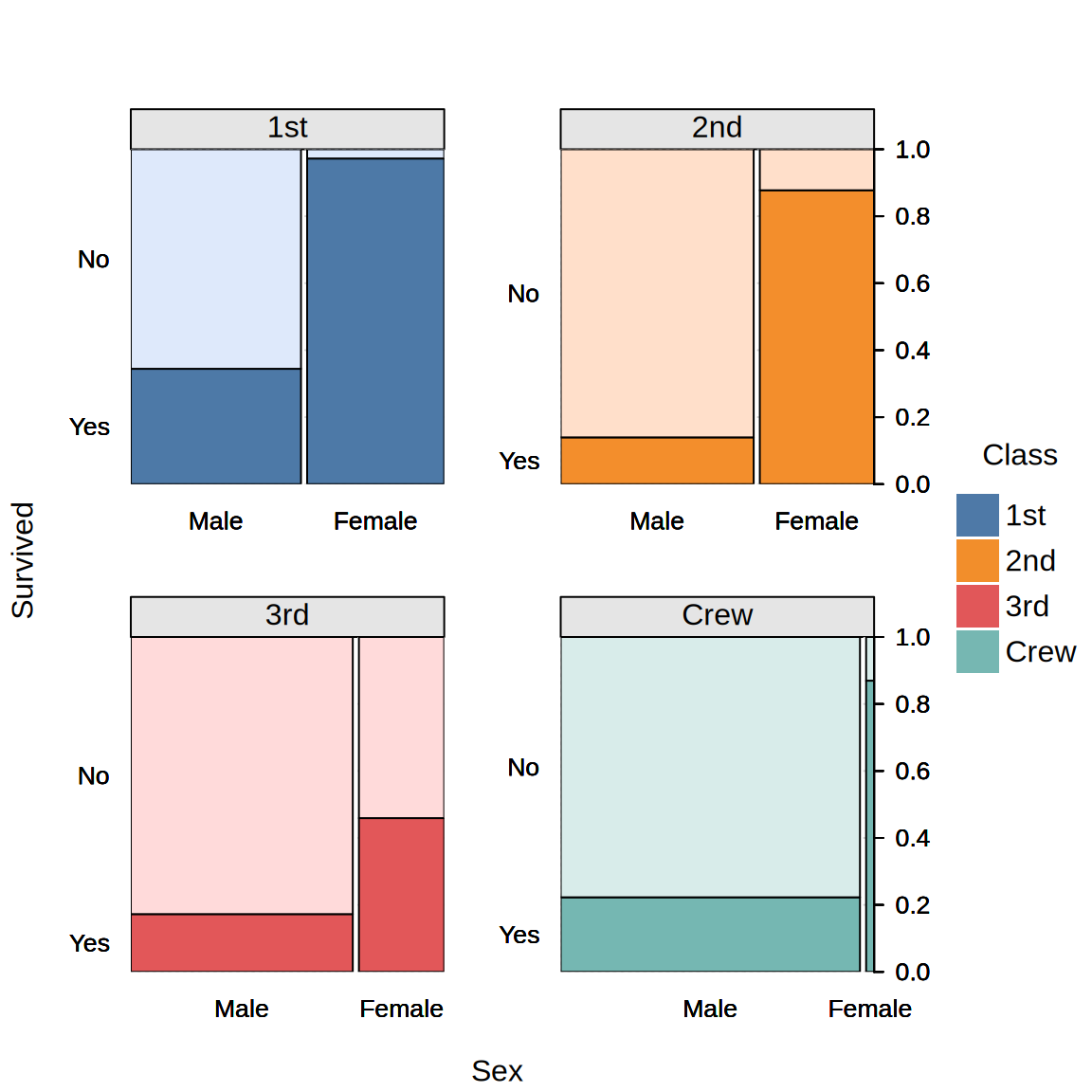
spineplot
Quickfire gallery
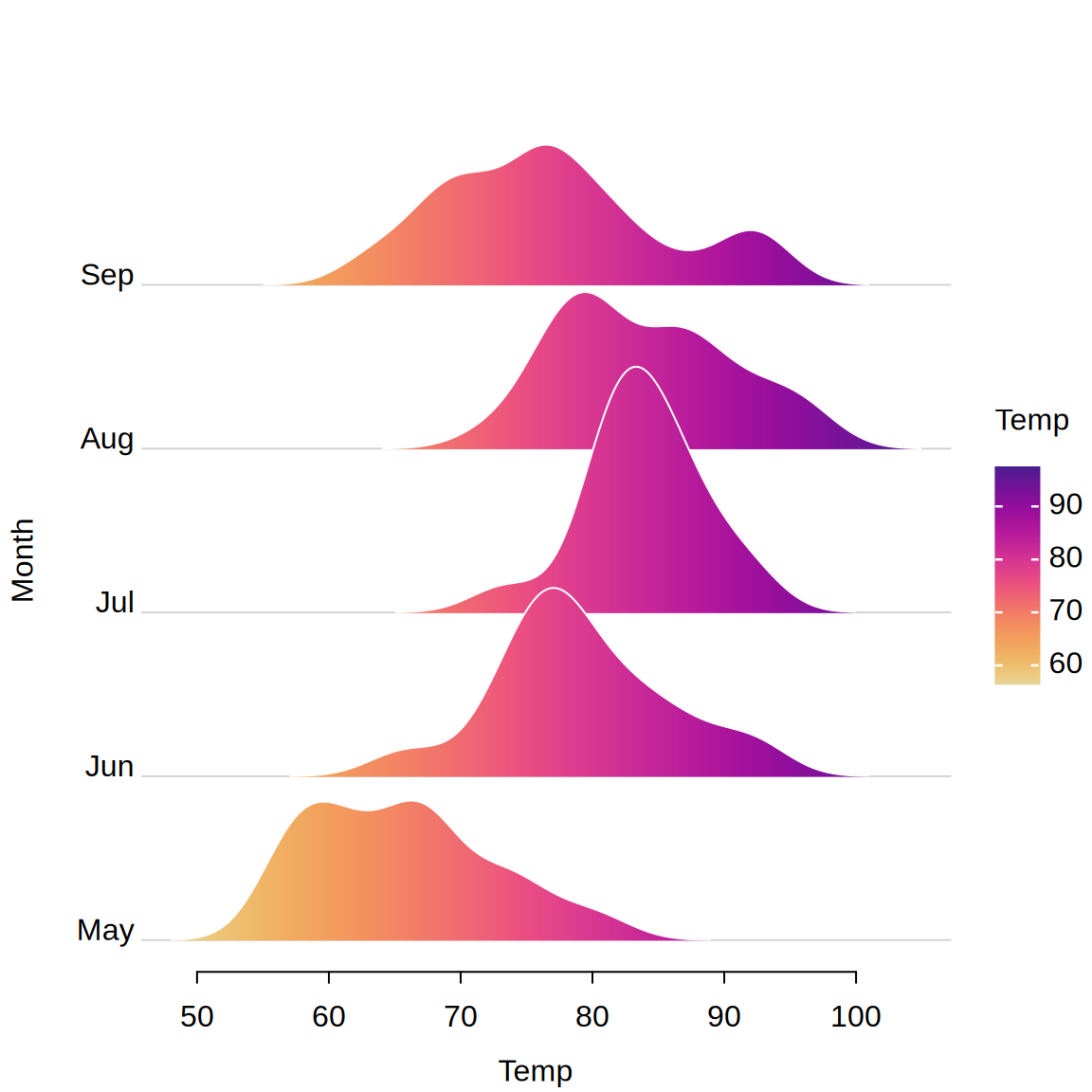
ridge plot
tinyplot
Learn more
Concise
The formula API gives bang for buck
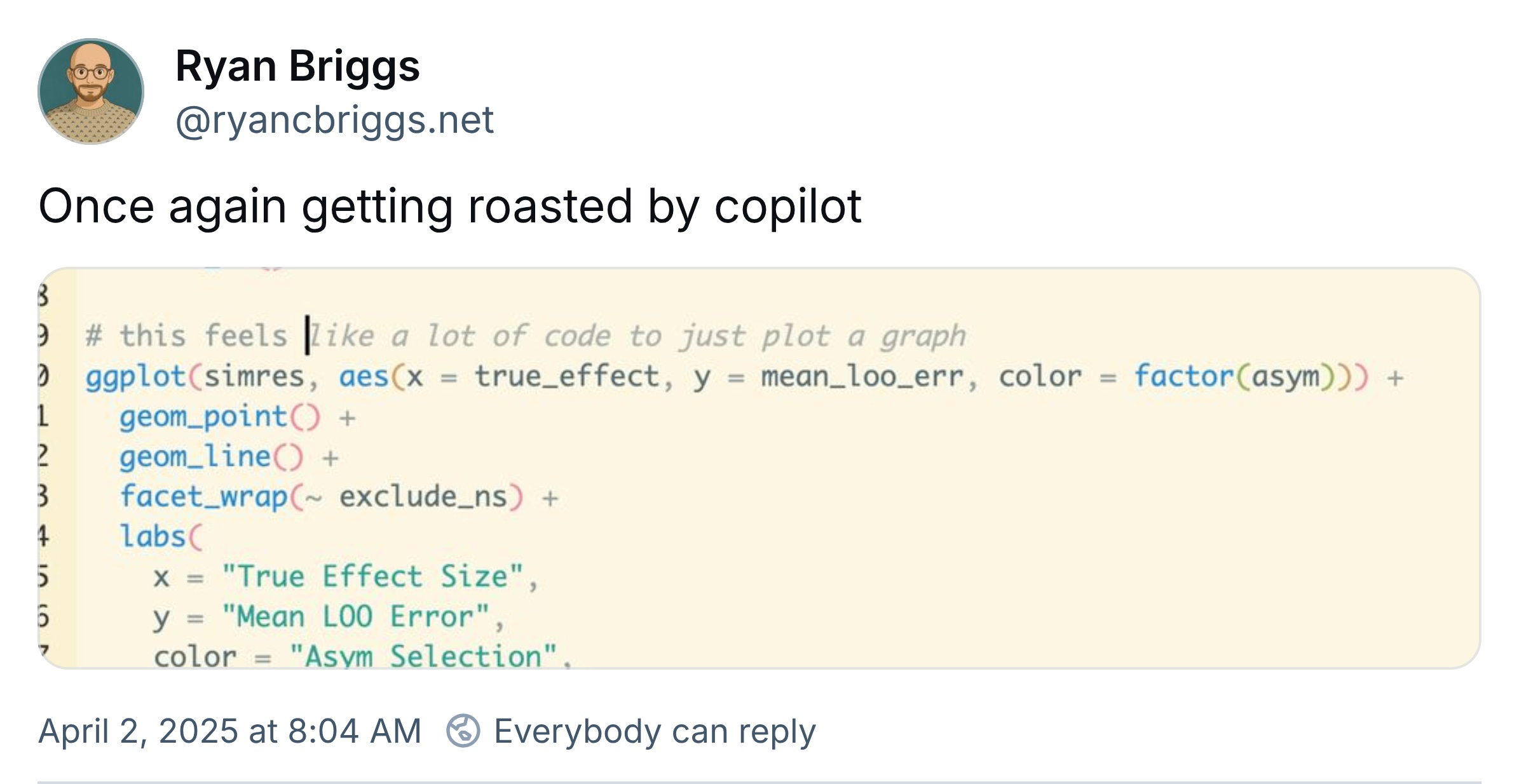
P.S. Thanks to Ryan for letting me use this screenshot.
Concise
Concision is even starker vs. vanilla base plot
Layering gotchas
Scaling is fixed by the first layer
This is a limitation of graphics “canvas” logic. (Workarounds: Change layer order, or use x/ylim.)