library(tinyplot)

aq = transform(
  airquality,
  Month = factor(Month, labels = month.abb[unique(Month)]),
  Hot = Temp > median(Temp)
)Plot types
A key feature of tinyplot is the type argument, which allows you to specify different kinds of plots. This tutorial will guide you through the various plot types available in tinyplot, demonstrating how the type argument can be used to to create a wide range of visualizations.
We will consider three categories of plot types:
- Base types
- tinyplot types
- Custom types
We will use the built-in airquality dataset for our examples:
Base types
The type argument in tinyplot supports all the standard plot types from base R’s plot function. These are specified using single-character strings.
"p"(Points): Produces a scatter plot of points. This is (usually) the default plot type."l"(Lines): Produces a line plot."b"(Points and Lines): Combines points and lines in same the plot."c"(Empty Points Joined by Lines): Plots empty points connected by lines."o"(Overplotted Points and Lines): Overlaps points and lines."s"and"S"(Stair Steps): Creates a step plot."h"(Histogram-like Vertical Lines): Plots vertical lines resembling a histogram."n"(Empty Plot): Creates an empty plot frame without data.
For example, we can use "b" to create a plot with combined points and lines.
tinyplot(Temp ~ Day | Month, data = aq, type = "b", main = "Points and lines")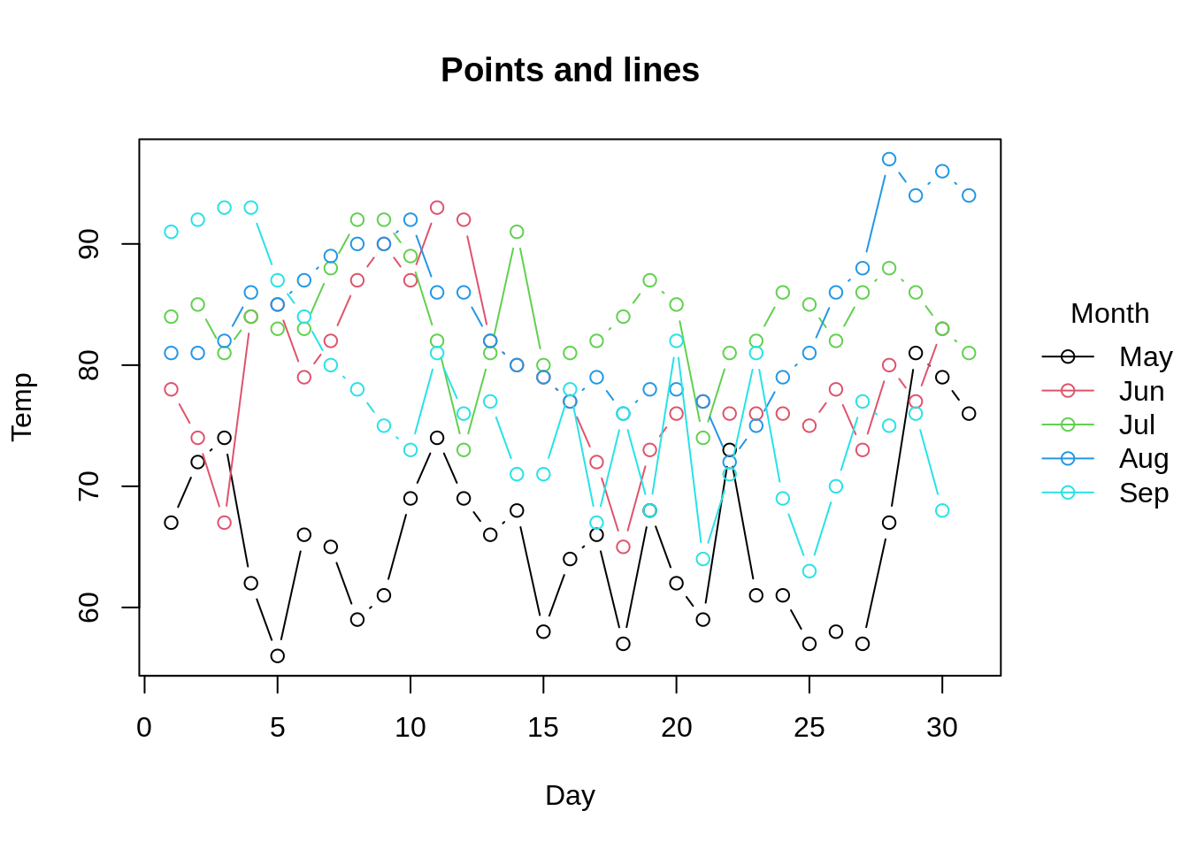
tinyplot types
Beyond the base types, tinyplot introduces additional plot types for more advanced visualizations. Each of these additional types are available either as a convenience string (with default behaviour) or a companion type_*() function (with options for customized behaviour).
Shapes
| string | function | description | docs |
|---|---|---|---|
"area" |
type_area() |
Plots the area under the curve from y = 0 to y = f(x). |
link |
"errorbar" |
type_errorbar() |
Adds error bars to points; requires ymin and ymax. |
link |
"l" / "b" / etc. |
type_lines() |
Draws lines and line-alike (same as base "l", "b", etc.) |
link |
"pointrange" |
type_pointrange() |
Combines points with error bars. | link |
"p" |
type_points() |
Draws points (same as base "p"). |
link |
"polygon" |
type_polygon() |
Draws polygons. | link |
"polypath" |
type_polypath() |
Draws a path whose vertices are given in x and y. |
link |
"rect" |
type_rect() |
Draws rectangles; requires xmin, xmax, ymin, and ymax. |
link |
"ribbon" |
type_ribbon() |
Creates a filled area between ymin and ymax. |
link |
"segments" |
type_segments() |
Draws line segments between pairs of points. | link |
"text" |
type_text() |
Adds text annotations to a plot. | link |
Visualizations
| string | function | description | docs |
|---|---|---|---|
"barplot" / "bar" |
type_barplot() |
Creates a bar plot. | link |
"boxplot" / "box" |
type_boxplot() |
Creates a box-and-whisker plot. | link |
"chull" |
type_chull() |
Draws convex hull(s) around grouped points. | link |
"density" |
type_density() |
Plots the density estimate of a variable. | link |
"ellipse" |
type_ellipse() |
Draws confidence ellipse(s) around grouped points. | link |
"histogram" / "hist" |
type_histogram() |
Creates a histogram of a single variable. | link |
"jitter" / "j" |
type_jitter() |
Jittered points. | link |
"qq" |
type_qq() |
Creates a quantile-quantile plot. | link |
"ridge" |
type_ridge() |
Creates a ridgeline (aka joy) plot. | link |
"rug" |
type_rug() |
Adds a rug to an existing plot. | link |
"spineplot" / "spine" |
type_spineplot() |
Creates a spine plot or spinogram. | link |
"violin" |
type_violin() |
Creates a violin plot. | link |
Models
| string | function | description | docs |
|---|---|---|---|
"loess" |
type_loess() |
Local regression curve. | link |
"lm" |
type_lm() |
Linear regression line. | link |
"glm" |
type_glm() |
Generalized linear model fit. | link |
"spline" |
type_spline() |
Cubic (or Hermite) spline interpolation. | link |
Functions
| string | function | description | docs |
|---|---|---|---|
"abline" |
type_abline() |
Line(s) with intercept and slope. | link |
"hline" |
type_hline() |
Horizontal line(s). | link |
"vline" |
type_vline() |
Vertical line(s). | link |
"function" |
type_function() |
Arbitrary function. | link |
"summary" |
type_summary() |
Summarizes y by unique values of x. |
link |
To see the difference between the convenience strings and their respective type_*() functional equivalents, let’s quickly walk through two examples.
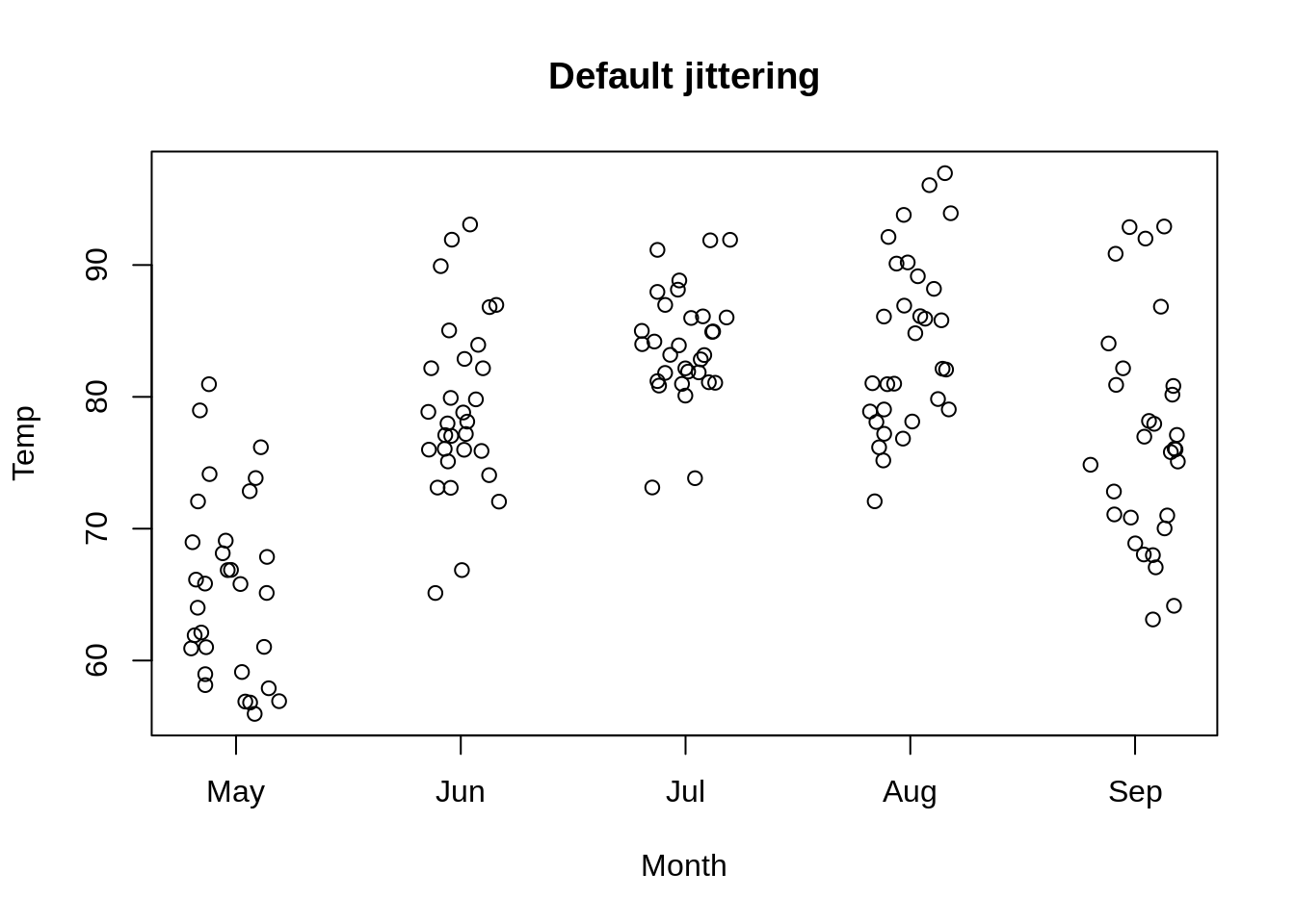
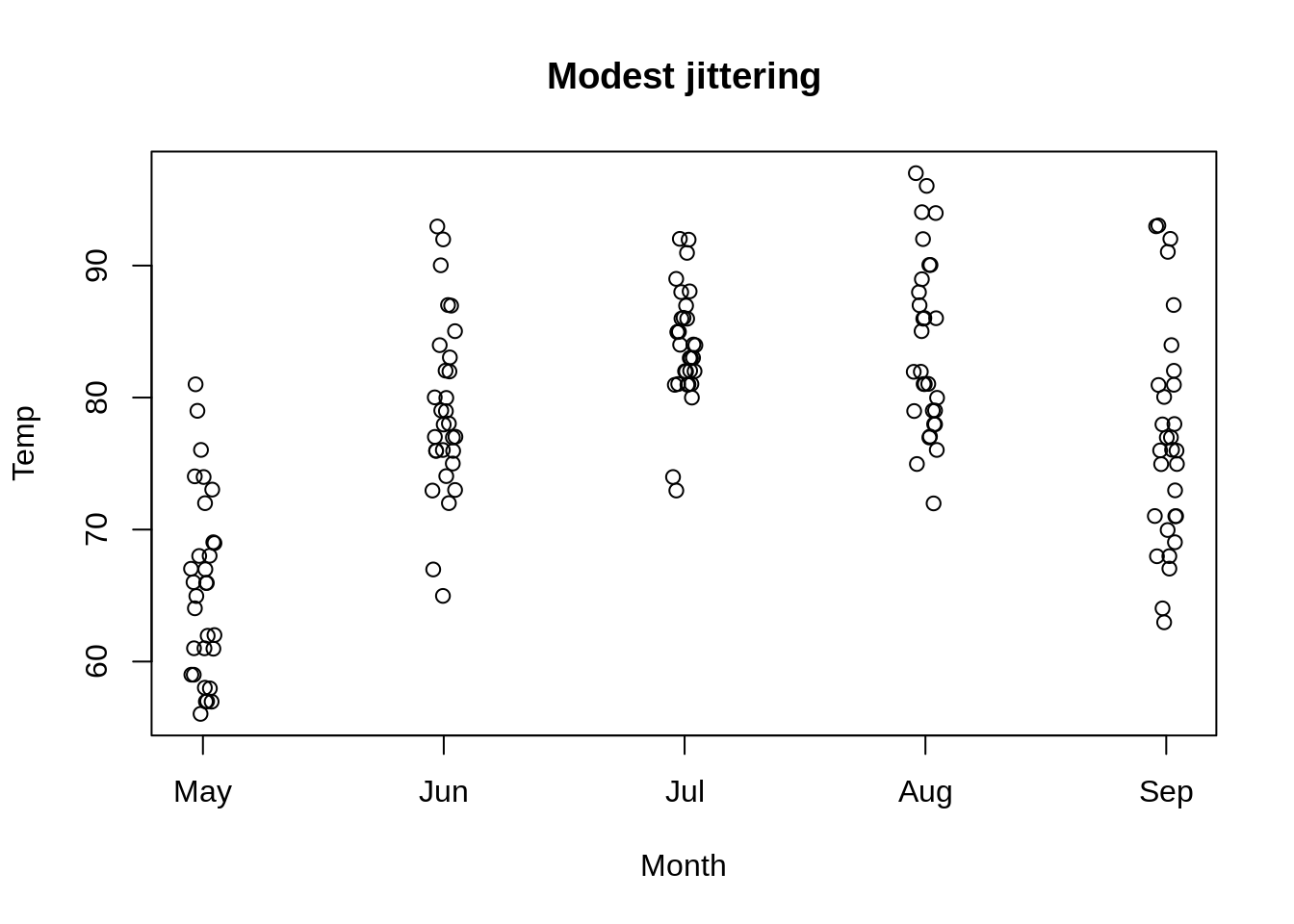
Example 1: jittering. We can add noise to data points using jittering. This allows us to avoid overplotting and can be useful to visualize discrete variables. On the left, we use the "jitter string shortcut with default settings. On the right, we use the type_jitter() function to reduce the amount of jittering.
tinyplot(
  Temp ~ Month, data = aq, main = "Default jittering",
  type = "jitter"
)
tinyplot(
  Temp ~ Month, data = aq, main = "Modest jittering",
  type = type_jitter(amount = 0.05)
)
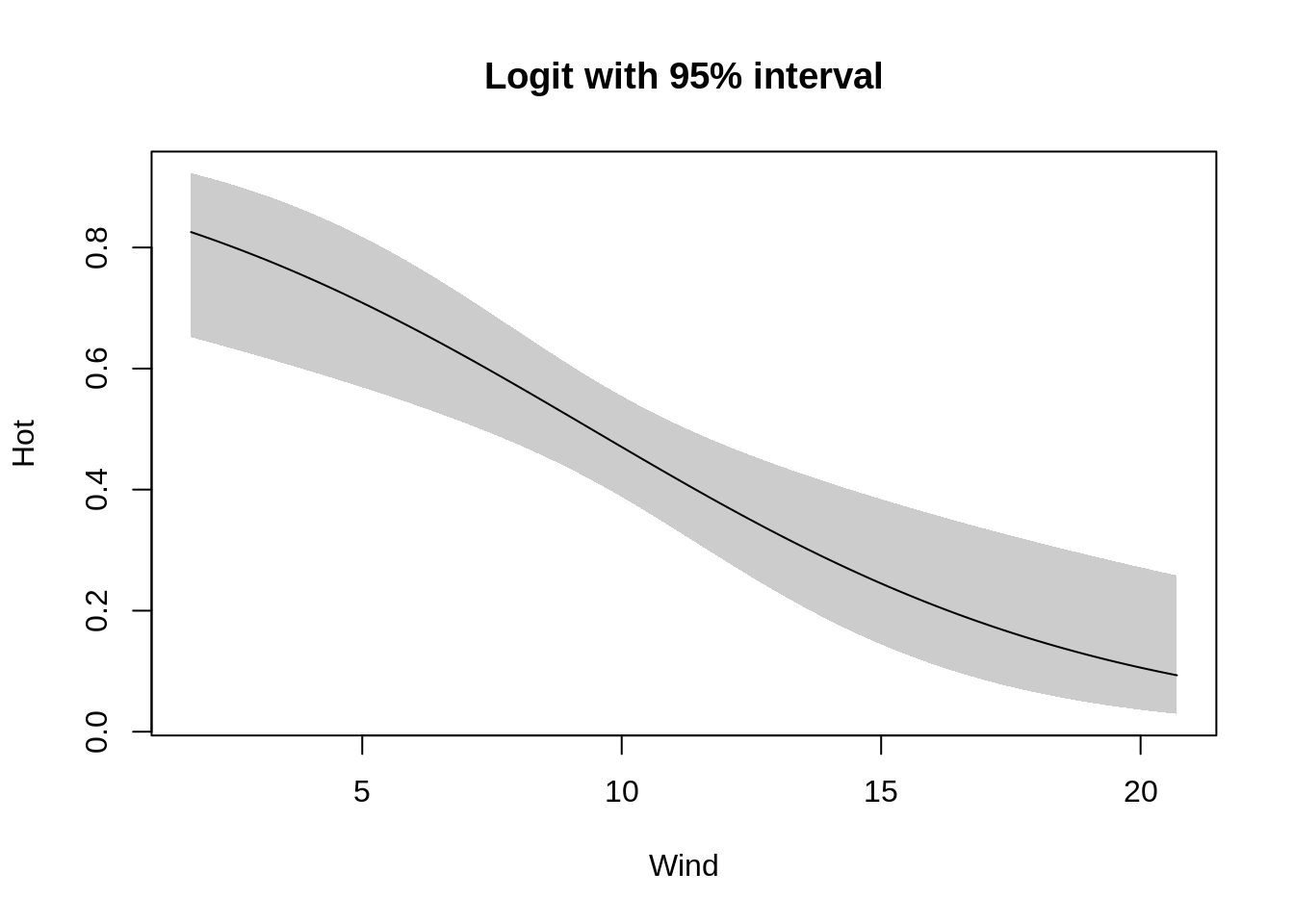
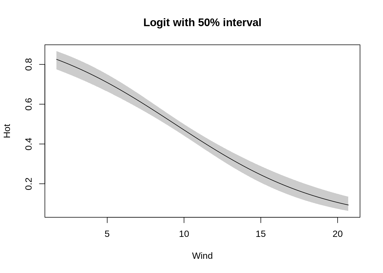
Example 2: Logit fit. In this example, we use type_glm() to fit a logistic regression model to the data, but with different confidence intervals.1
tinyplot(
  Hot ~ Wind, data = aq, main = "Logit with 95% interval",
  type = type_glm(family = "binomial")
)
tinyplot(
  Hot ~ Wind, data = aq, main = "Logit with 50% interval",
  type = type_glm(family = "binomial", level = 0.5)
)
To see what arguments are available for each type, simply consult the type-specific documentation.
?type_jitter
?type_glm
# etc
Finally, please note that all tinyplot types support grouping and faceting.
tinyplot(Temp ~ Wind | Month, data = aq, facet = "by", type = "lm")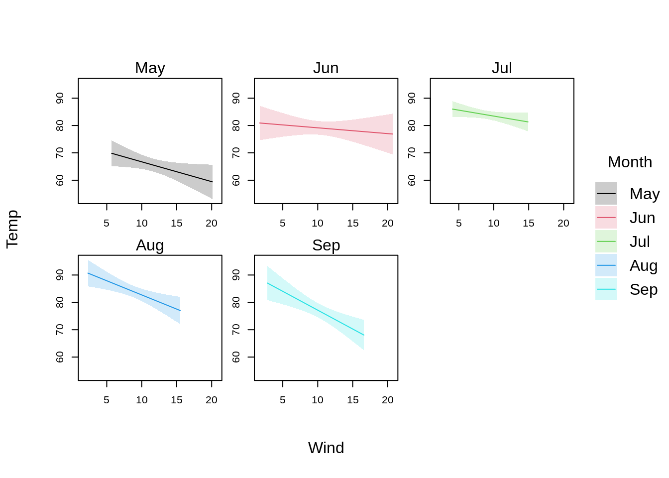
Custom types
It is easy to add custom types to tinyplot. Users who need highly customized plots, or developers who want to add support to their package or functions, only need to define their own type_<type>() function. Let’s start with a simple example to see how this works in practice.
A minimal example
Here is a minimal example of a custom type_log() that logs both x and y before plotting points.
type_log = function(base = exp(1)) {

  # data tranformation function
  data_log = function() {
    fun = function(settings, ...) {
      # extract raw datapoints from settings environment
      datapoints = settings$datapoints

      # transform (log) the data
      datapoints$x = log(datapoints$x, base = base)
      datapoints$y = log(datapoints$y, base = base)
      datapoints = datapoints[order(datapoints$x), ]

      # re-assign modified datapoints back to settings
      settings$datapoints = datapoints
    }
    return(fun)
  }

  # drawing function
  draw_log = function() {
    fun = function(ix, iy, icol, ...) {
      points(
        x = ix,
        y = iy,
        col = icol
      )
    }
    return(fun)
  }

  # return object (list)
  out = list(
    data = data_log(),
    draw = draw_log(),
    name = "p" # fallback behaviour same as "p" type (e.g., legend defaults)
  )
  class(out) = "tinyplot_type"
  return(out)

}
To use, simply pass to type = type_log(<args>) as per as normal.
tinyplot(mpg ~ wt | factor(am), data = mtcars,
  type = type_log(), main = "Ln (natural logarithm)")
tinyplot(mpg ~ wt | factor(am), data = mtcars,
  type = type_log(base = 10), main = "Log (base 10)")

How it works
As illustrated by our minimal example, custom tinyplot types require three key functions:
type_<type>(): The main wrapper function that users will call. It should accept any type-specific arguments that users will need to adjust the final plot (e.g., here:base). More importantly, it must return a list of class"tinyplot_type"and contain three elements:data: A data transformation function (see below)draw: A drawing function (see below)name: The name of the underlying plot type (this can be anything, but think of it as a convenient way to inherit default/fallback behaviour from an existing plot type)
data_<type>(): A function factory that returns a data transformation function:- Required arguments:
settingsand... settingsis an environment containing plot data and parameters, includingdatapoints(a data frame withx,y,by, etc.),legend_args(a list of legend customizations), and many other internal parameters (see Appendix: Available settings below for a complete list).- Should modify
settingsin-place (e.g.,settings$datapoints = ...) - Does not need to return anything
- Required arguments:
draw_<type>(): A function factory that returns a drawing function:- Required arguments:
... - Available arguments:
ix,iy,ixmin,ixmax,iymin,iymax,icol,ibg,ipch,ilty,ilwd,icex, and others - The
iprefix indicates data for a single group (when using|grouping or facets) - Should call base R graphics functions (e.g.,
points(),lines(),polygon()) to render the plot
- Required arguments:
The key insight is that data_*() transforms the data once, while draw_*() is called repeatedly for each group or facet.
Pro tip: Re-use existing plot types
Rather than code up all of the internals for a custom type from scratch, users are strongly encouraged to re-use the scaffolding for existing types. One of the easiest ways to do this—which we use repeatedly in the main tinyplot codebase—is by “delegating” to an existing type at the end of the data_<type> function. Again, this is perhaps easier seen than explained, so consider an alternate version of our previous type_log() function.
type_log_redux = function(base = exp(1)) {

  # data tranformation function
  data_log = function() {
    fun = function(settings, ...) {
      datapoints = settings$datapoints

      datapoints$x = log(datapoints$x, base = base)
      datapoints$y = log(datapoints$y, base = base)
      datapoints = datapoints[order(datapoints$x), ]

      settings$datapoints = datapoints

      # re-assign/delegate to "p" type
      settings$type = "p"
    }
    return(fun)
  }

  # return object (list)
  out = list(
    data = data_log(),
    draw = NULL, # NULL => fall back to default type (now "p") drawing function
    name = "log"
  )
  class(out) = "tinyplot_type"
  return(out)

}
The key differences from our original type_log function are:
settings$type = "p"(re-assign the type at the end ofdata_log())draw = NULL(drop the dedicateddraw_log()function entirely; will fall back todraw_points()internally now)
This “redux” version is obviously shorter than our original version, since we can skip the custom draw_log() section. But re-using existing tinyplot scaffolding brings added benefits beyond code concision. In particular, it guarantees that all of the functionality from an existing type will be made available to your custom type. For example, in our first type_log() function we didn’t account for the fact that users might want to adjust groups by other aesthetics (e.g, pch), whereas we get this for free in type_log_redux().
tinyplot(mpg ~ wt | factor(am), data = mtcars,
  pch = "by",
  type = type_log(), main = "type_log")
tinyplot(mpg ~ wt | factor(am), data = mtcars,
  pch = "by",
  type = type_log_redux(), main = "type_log_redux")

Moral of the story: be lazy and re-use existing tinyplot scaffolding wherever possible; especially drawing functions.
More examples
The tinyplot source code contains many examples of type constructor functions that should provide a helpful starting point for custom plot types. Each built-in tinyplot type is itself implemented as a custom type, so you can see real-world examples of varying complexity. For example, take a look at the type_points.R or type_area.R code. (The latter provides an example where we delegate to the type_ribbon drawing code.)
Beyond that, the tinyplot team are always happy to help guide users on how to create their own types. Just let us know by raising an issue on our GitHub repo.
Appendix: Available settings
To see what objects and parameters are available in the settings environment, we can create a simple type_error() function that stops with the names of all available settings:
type_error = function() {
  data_error = function() {
    fun = function(settings, ...) {
      stop(paste(sort(names(settings)), collapse = ", "))
    }
    return(fun)
  }

  out = list(
    data = data_error()
  )
  class(out) = "tinyplot_type"
  return(out)
}

tinyplot(mpg ~ wt, data = mtcars, type = type_error())
Error in `settings$type_data()`:
! add, alpha, axes, bg, bubble, bubble_alpha, bubble_bg_alpha, bubble_pch, by, by_dep, call, cap, cex, cex_dep, col, datapoints, dodge, dots, draw, facet, facet_attr, facet_by, facet_dep, facet.args, file, fill, flip, frame.plot, group_offsets, height, labels, legend, legend_args, lighten, log, lty, lwd, null_by, null_facet, null_palette, null_xlim, null_ylim, offsets_axis, palette, pch, rev_x, rev_y, ribbon.alpha, sub, type, type_data, type_draw, type_info, type_name, weights, weights_used, width, x, x_by, x_dep, xaxb, xaxl, xaxs, xaxt, xlab, xlabs, xlim, xmax, xmax_dep, xmin, xmin_dep, y, y_dep, yaxb, yaxl, yaxs, yaxt, ygroup, ylab, ylabs, ylim, ymax, ymax_dep, ymin, ymin_depAs we can see, the settings environment contains many parameters that custom types can use as inputs or modify as needed.
Footnotes
Note: If we simply specified the
"glm"convenience string on its own, we’d get a linear fit since the default family isgaussian.↩︎