Lines plot type

Description

Type function for plotting lines.

Usage

type_lines(
  type = "l",
  dodge = 0,
  fixed.dodge = FALSE,
  xlevels = NULL,
  xord = NULL
)

Arguments

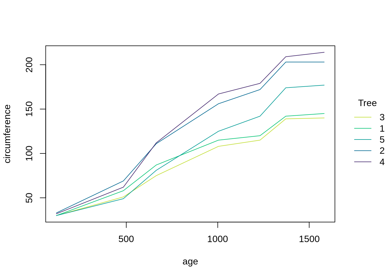
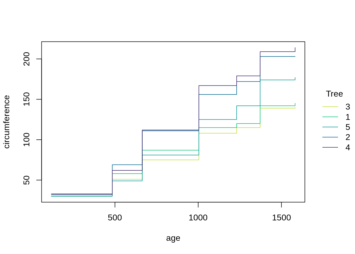
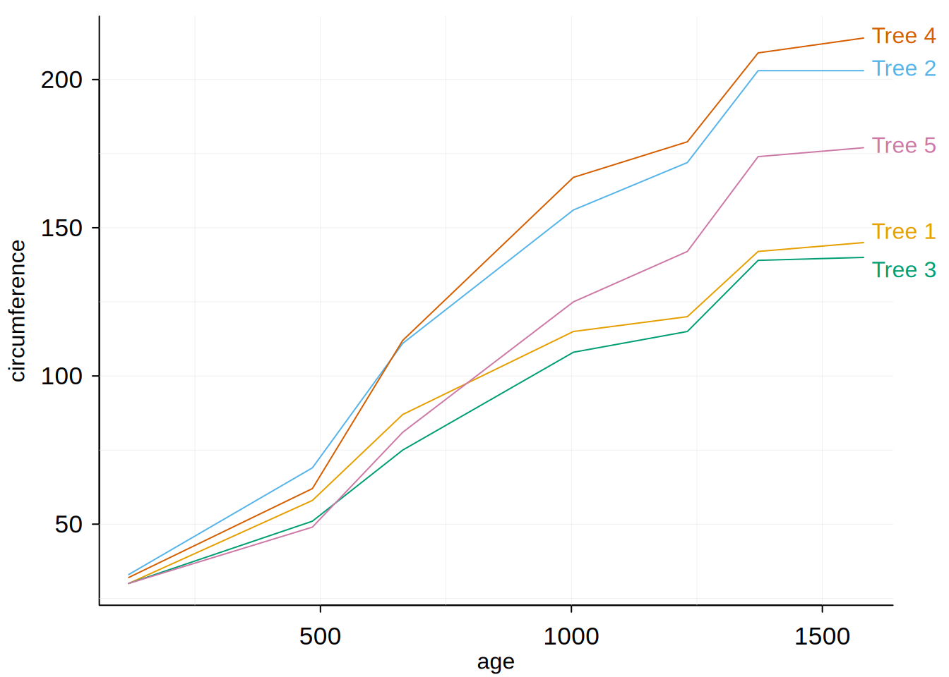
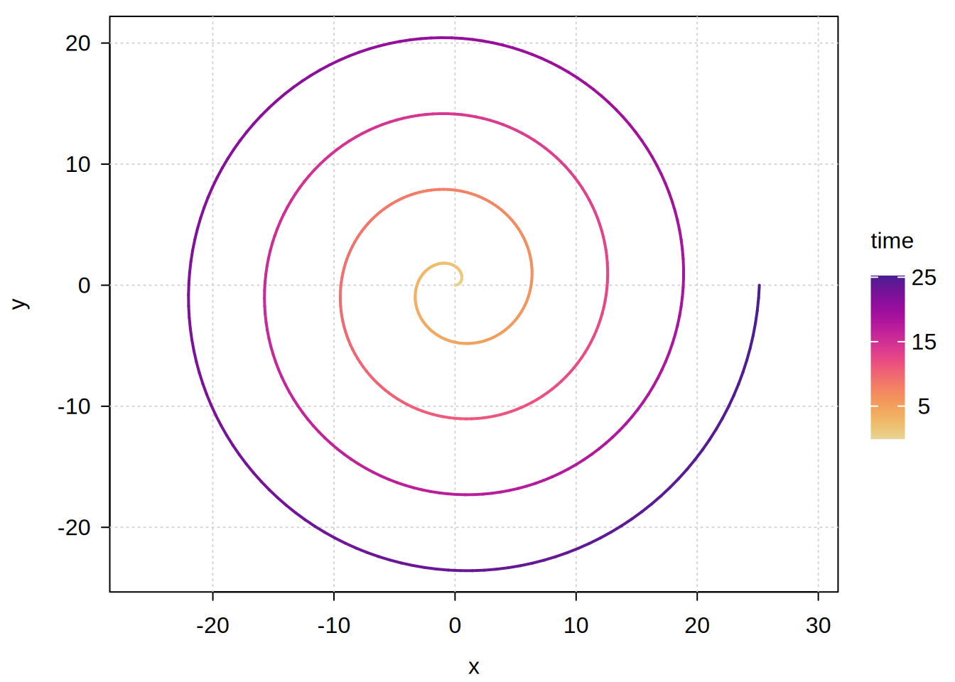
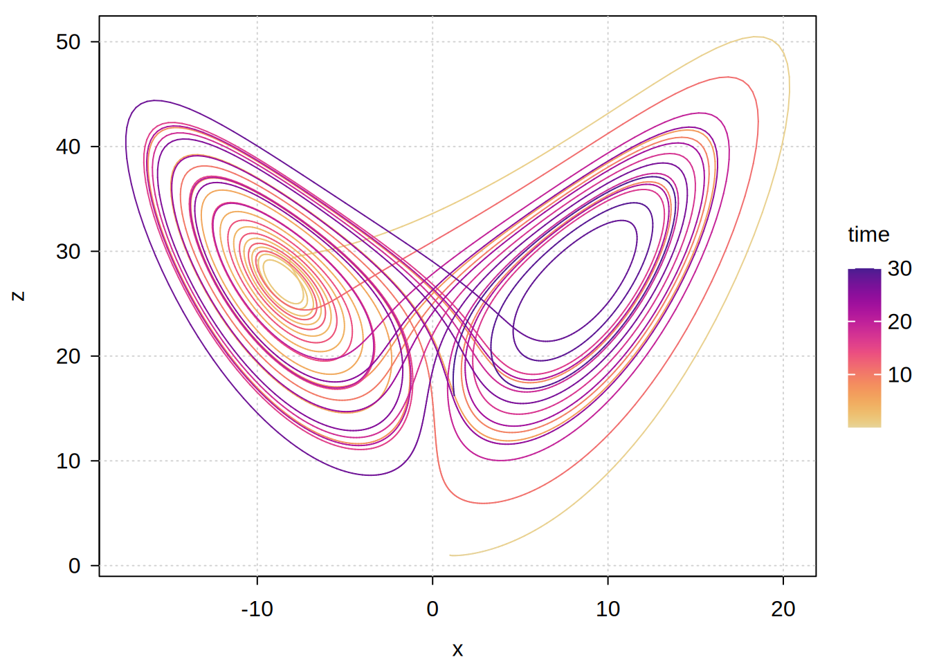
type	1-character string giving the type of plot desired. The following values are possible, for details, see plot: “p” for points, “l” for lines, “b” for both points and lines, “c” for empty points joined by lines, “o” for overplotted points and lines, “s” and “S” for stair steps and “h” for histogram-like vertical lines. Finally, “n” does not produce any points or lines.
dodge	Adjustment parameter for dodging overlapping points or ranges in grouped plots along the x-axis (or y-axis for flipped plots). Either: numeric value in the range [0,1). Note that values are scaled relative to the spacing of x-axis breaks, e.g. dodge = 0.1 places the outermost groups one-tenth of the way to adjacent breaks, dodge = 0.5 places them midway between breaks, etc. Values < 0.5 are recommended. logical. If TRUE, the dodge width is calculated automatically based on the number of groups (0.1 per group for 2-4 groups, 0.45 for 5+ groups). If FALSE or 0, no dodging is performed. Default value is 0 (no dodging). While we do not check, it is strongly recommended that dodging only be used in cases where the x-axis comprises a limited number of discrete breaks.
fixed.dodge	Logical. If FALSE (default), dodge positions are calculated independently for each x value, based only on the groups present at that position. If TRUE, dodge positions are based on all groups, ensuring "fixed" spacing across x-axis breaks (i.e., even if some groups are missing for a particular x value).
xlevels, xord	arguments controlling the order of the (categorical) x variable, and hence of the x-axis. Supply one or the other; if both arguments are provided, xlevels takes precedence and xord is silently ignored. xlevels specifies the levels literally, either a character vector of level names in the desired order (e.g., c(“C”, “B”, “A”)), or a numeric vector of the corresponding level indexes (e.g. 3:1). xord instead accepts a keyword or custom function, which then derives the order from the data. Options are: “desc” and “asc” rank the categories by their mean y value, largest or smallest first. (Long forms like “descending” and “increasing” are also accepted.) “minvar” ranks them by the variance of those values, lowest first. “asis” or “rev” permute the existing levels without consulting the data at all. The former takes the categories in the order that they appear in the data, while the latter reverses the current level order. a custom function that determines both the ranking statistic and its direction. The statistic is always sorted ascending, so function(y) -median(y) ranks by median, largest first. Note that x is only reordered when it is categorical (i.e., factor or character). A numeric x is plotted at its own values and cannot be reordered, so supplying either argument there is ignored with a warning. Each argument defaults to NULL, i.e. keep the existing factor levels.

Categorical axes

Like the other plot types, type_lines() places categorical (factor or character) data according to the factor levels. Character variables are coerced with factor() and so end up in alphabetical order. To order the categories by their appearance in the data instead, use xord = “asis”, or set the levels explicitly, e.g. factor(x, levels = unique(x)).

Note that the lines themselves are always drawn in the order that the rows arrive in, exactly as base lines() does. Categories whose level order differs from their row order will therefore produce a zig-zag, just as an unsorted numeric x-variable would.

Examples

library("tinyplot")

# "l" type convenience character string
tinyplot(circumference ~ age | Tree, data = Orange, type = "l")

# Use `type_lines()` to pass extra arguments for customization
tinyplot(circumference ~ age | Tree, data = Orange, type = type_lines(type = "s"))

# Direct legend labels are a good option for grouped lined plots (assuming
# there aren't too many groups and the data are sorted along the x-axis)
tinyplot(
  circumference ~ age | Tree, data = Orange, type = "l",
  legend = "direct"
)

# Fancier version(s) that use a theme and repel overlapping labels
Orange2 = transform(Orange, Tree = paste("Tree", Tree))
tinyplot(
  circumference ~ age | Tree, data = Orange2, type = "l",
  legend = list("direct", repel = TRUE), # auto repel
  theme = "socviz"
)

tinyplot(
  circumference ~ age | Tree, data = Orange2, type = "l",
  legend = list("direct", nudge_y = c("Tree 1" = 3, "Tree 3" = -5)), # manual
  theme = "socviz"
)

# A continuous `by` variable is also supported (as of tinyplot v0.8.0).
# This is particularly useful for trajectories, where a third variable (often
# time) orders the path.
time = seq(0, 8*pi, length.out = 600)
spiral = data.frame(time = time, x = time * cos(time), y = time * sin(time))
tinyplot(
  y ~ x | time, data = spiral,
  type = "l",
  lwd = 2, asp = 1, # optional args
  theme = "clean"
)

# The canonical time-path example: the x-z projection of a Lorenz attractor.
step = function(p, i) {
  p + 0.005 * c(
    10 * (p[2] - p[1]),
    p[1] * (28 - p[3]) - p[2],
    p[1] * p[2] - 8/3 * p[3]
  )
}
lz = do.call(rbind, Reduce(step, 1:6000, c(1, 1, 1), accumulate = TRUE))
lorenz = data.frame(time = seq_len(nrow(lz)) * 0.005, x = lz[, 1], z = lz[, 3])
tinyplot(z ~ x | time, data = lorenz, type = "l", theme = "clean")