bw
|
the smoothing bandwidth to be used, see density for details and options.
|
joint.bw
|
character string indicating whether (and how) the smoothing bandwidth should be computed from the joint data distribution when there are multiple subgroups. The options are “mean” (the default), “full”, and “none”. Also accepts a logical argument, where TRUE maps to “mean” and FALSE maps to “none”. See the "Bandwidth selection" section below for a discussion of practical considerations.
|
adjust
|
the bandwidth used is actually adjust*bw. This makes it easy to specify values like ‘half the default’ bandwidth.
|
kernel
|
a character string giving the smoothing kernel to be used. This must partially match one of “gaussian”, “rectangular”, “triangular”, “epanechnikov”, “biweight”, “cosine” or “optcosine”, with default “gaussian”, and may be abbreviated to a unique prefix (single letter).
“cosine” is smoother than “optcosine”, which is the usual ‘cosine’ kernel in the literature and almost MSE-efficient. However, “cosine” is the version used by S.
|
n
|
the number of equally spaced points at which the density is to be estimated. When n > 512, it is rounded up to a power of 2 during the calculations (as fft is used) and the final result is interpolated by approx. So it almost always makes sense to specify n as a power of two.
|
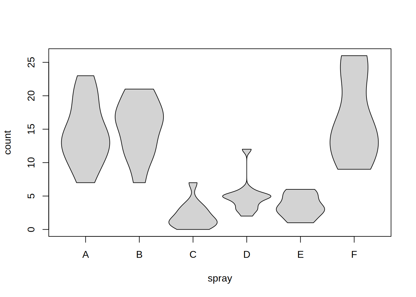
trim
|
logical indicating whether the violins should be trimmed to the range of the data. Default is FALSE.
|
width
|
numeric (ideally in the range [0, 1], although this isn’t enforced) giving the normalized width of the individual violins.
|
lighten
|
logical. Should the fills use a lighter, opaque tint of the series colour(s)? Default is TRUE, which keeps single- and multi-group displays consistent and lets the fill read cleanly over grid lines. Set to FALSE to use the fully-saturated palette colour(s) instead.
|