Set or Reset Plot Themes for tinyplot

Description

The tinytheme function sets or resets the theme for plots created with tinyplot. Themes control the appearance of plots, such as text alignment, font styles, axis labels, and even dynamic margin adjustment to reduce whitespace.

Usage

tinytheme(
  theme = c("default", "basic", "dynamic", "clean", "clean2", "bw", "linedraw",
    "classic", "minimal", "ipsum", "ipsum2", "dark", "socviz", "broadsheet", "nber",
    "web", "heatmap", "ridge", "ridge2", "tufte", "float", "void"),
  ...,
  register = NULL
)

Arguments

theme	A character string specifying the name of the theme to apply. Themes are arranged in an approximate hierarchy, adding or subtracting elements in the order presented below. Note that several themes are dynamic, in the sense that they attempt to reduce whitespace in a way that is responsive to the length of axes labels, tick marks, etc. These dynamic plots are marked with an asterisk (*) below. 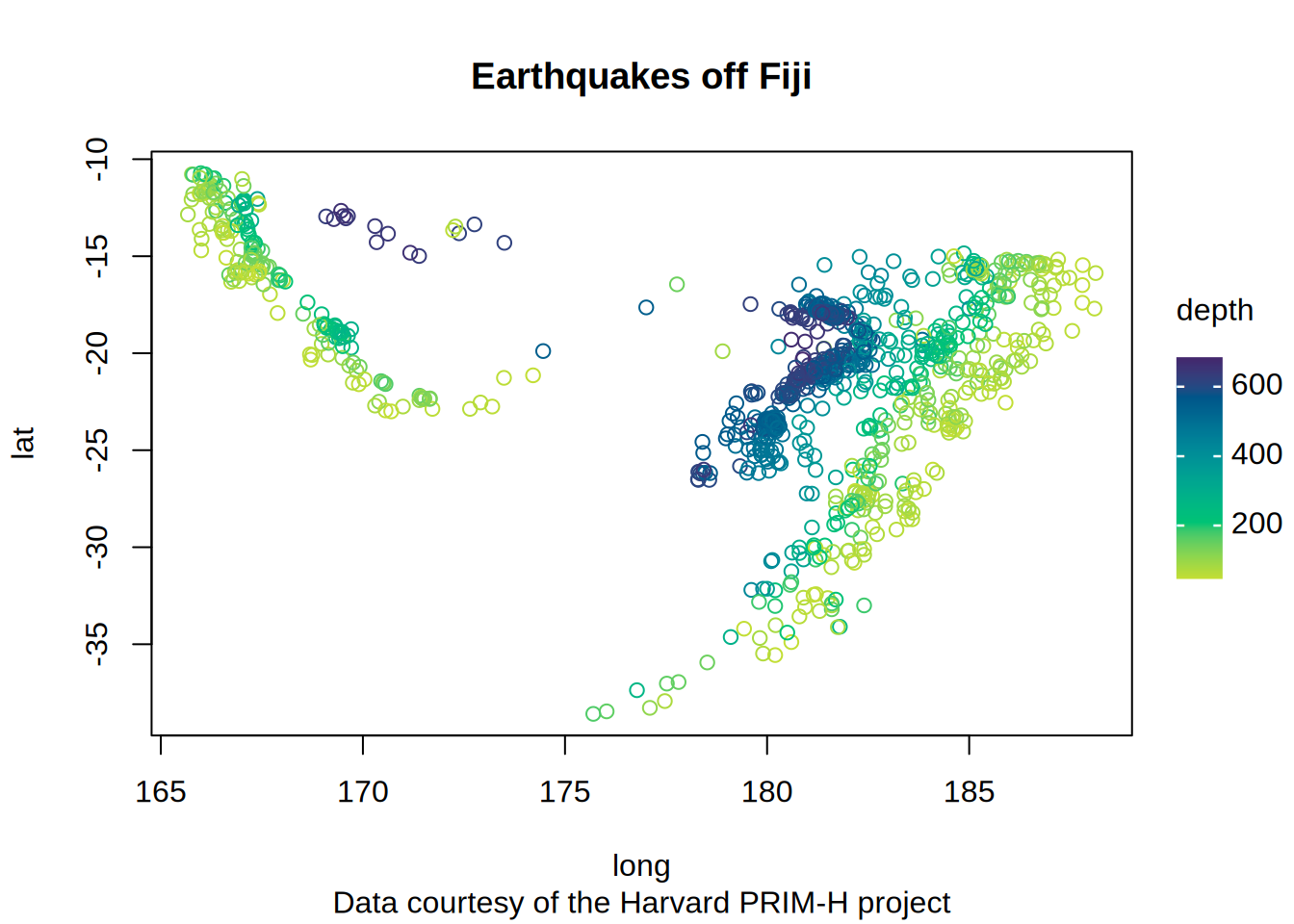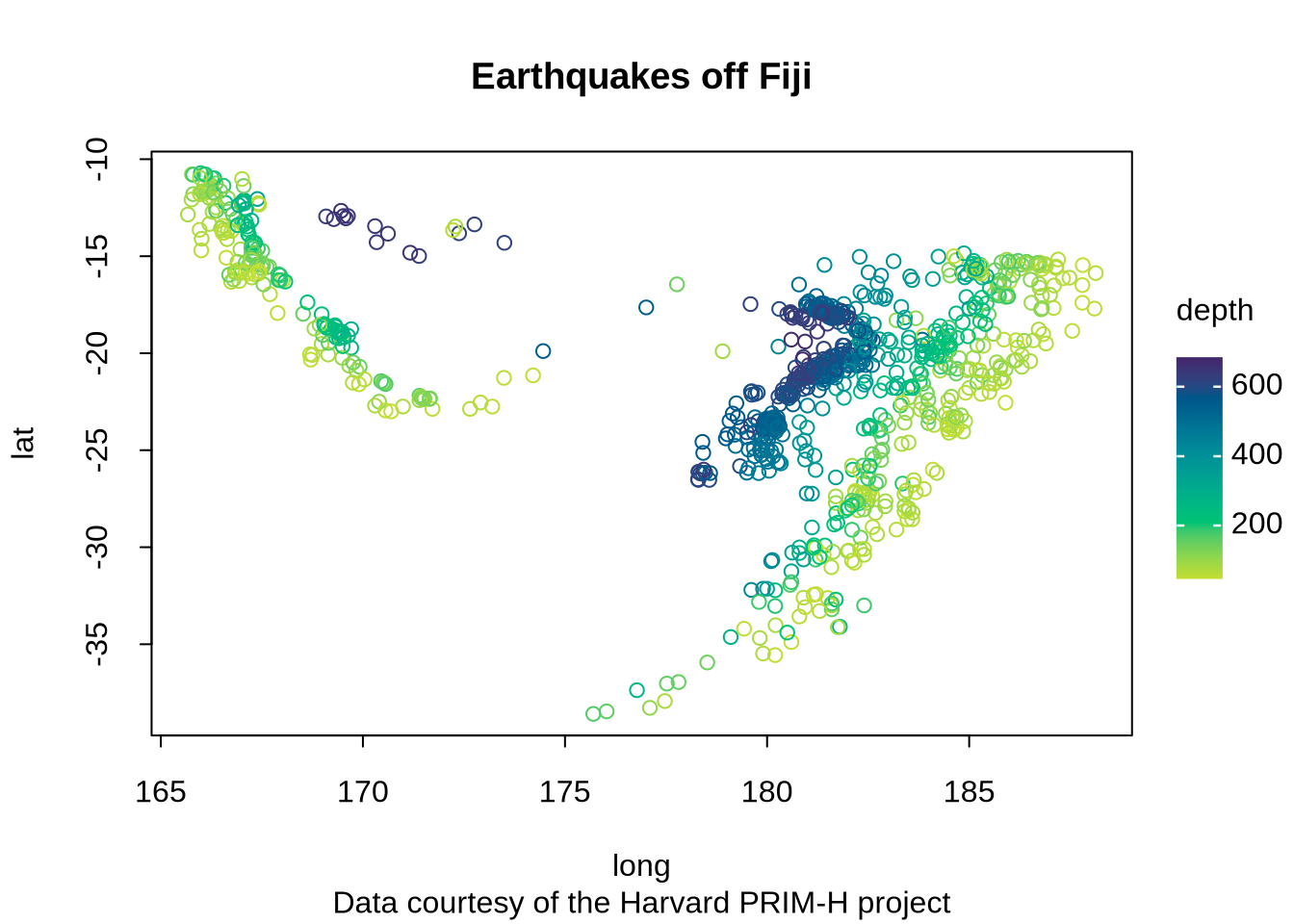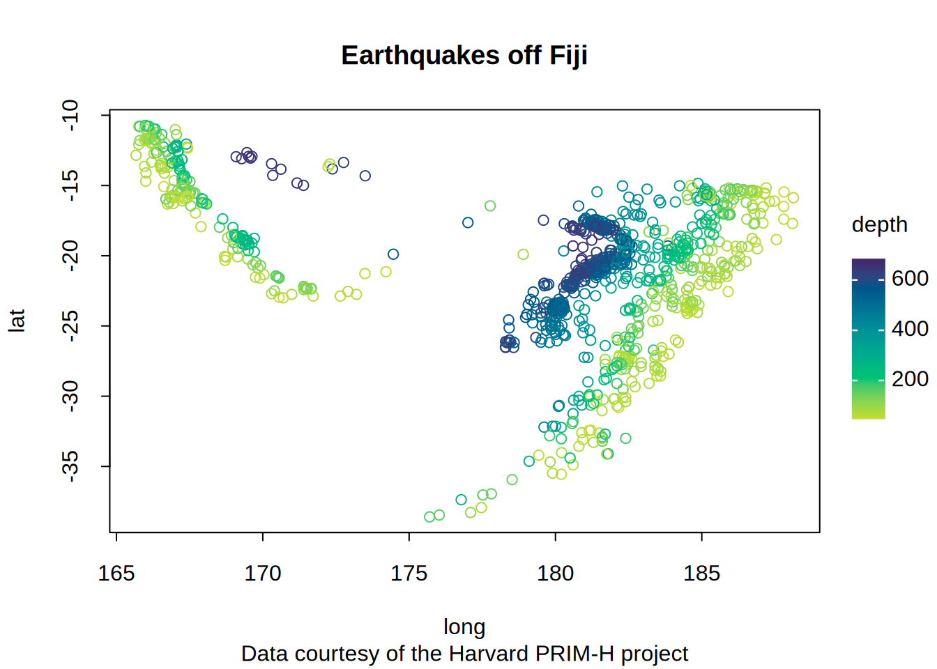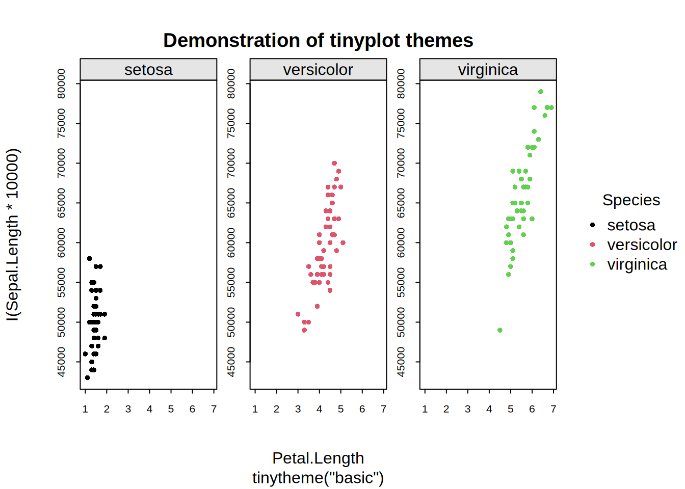“default”: inherits the user’s default base graphics settings. “basic”: light modification of “default”, only adding filled points, a panel background grid, and light gray background to facet titles. “dynamic” (*): builds on “basic” by enabling dynamic margin adjustment with tighter default margins, horizontal axis labels, and the subtitle moved above the plotting area. Turns off the panel grid. Provides the foundation for all other dynamic themes and is a good starting point for users who wish to build custom dynamic themes. 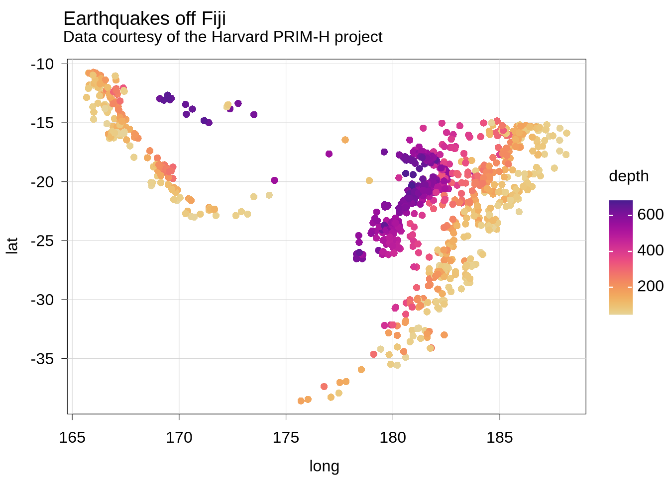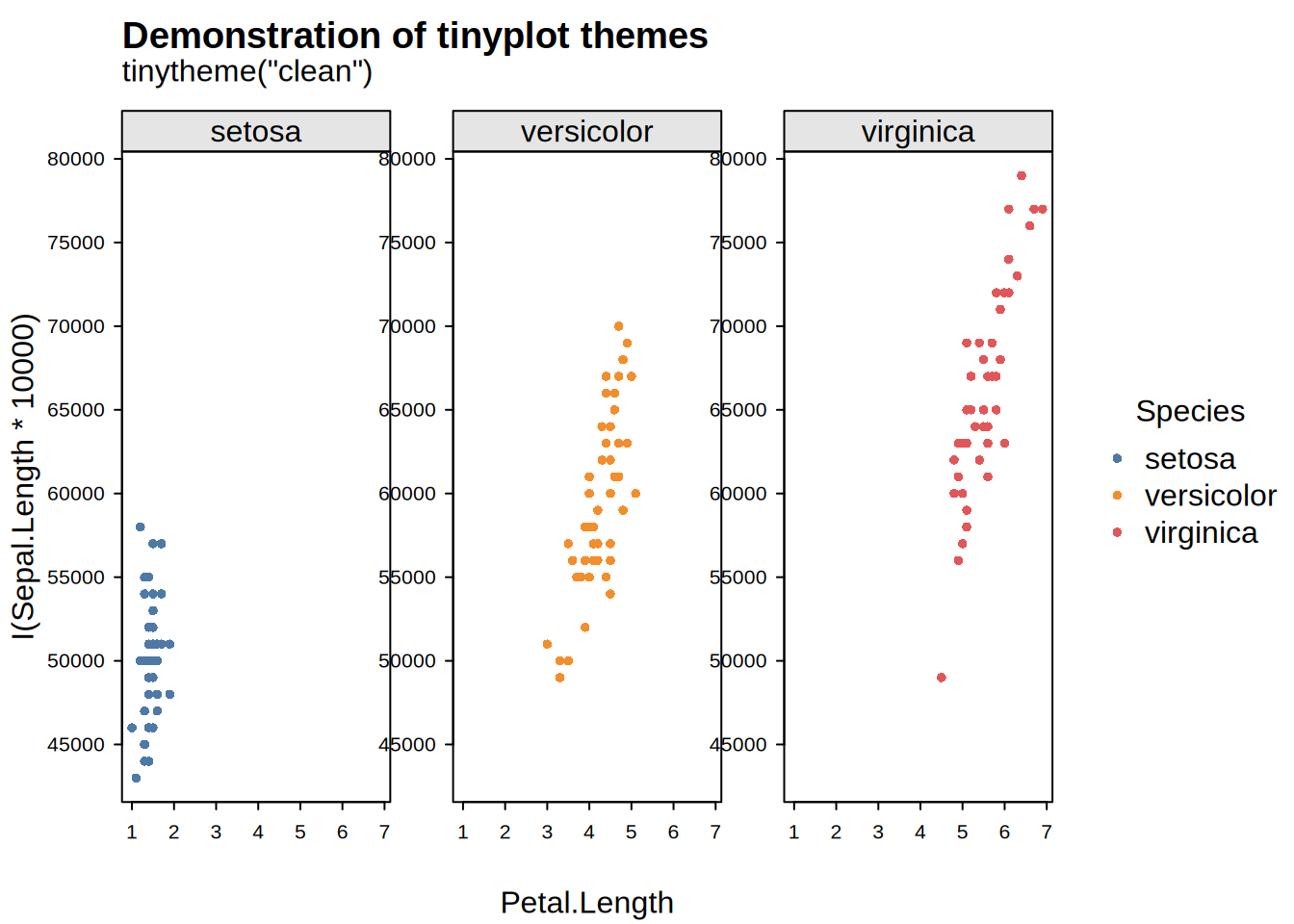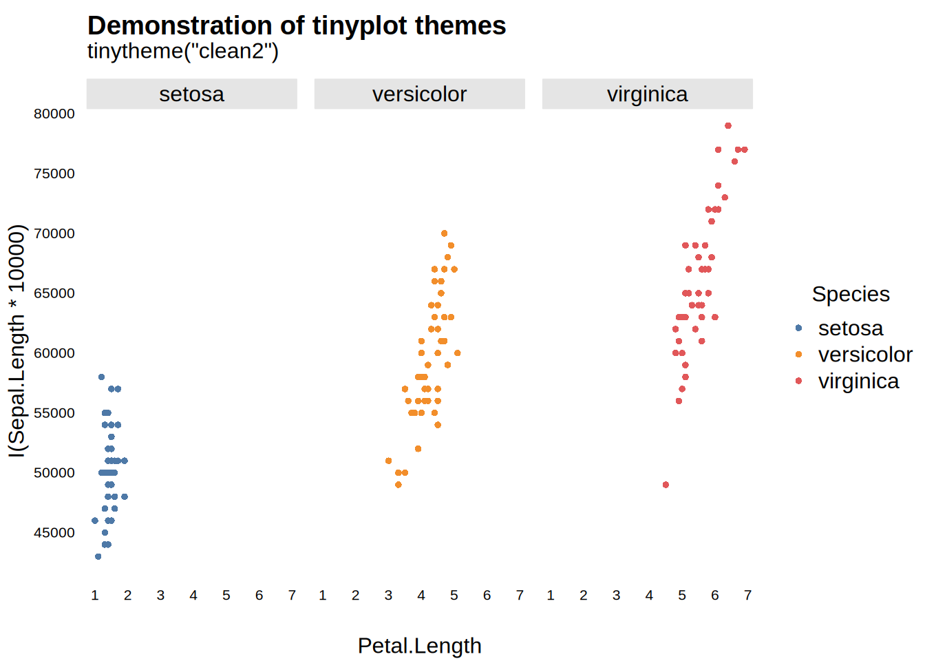“clean” (*): builds on “dynamic” by re-enabling the panel background grid and setting different default palettes ("Tableau 10" for discrete colors and "agSunset" for gradient colors). “clean2” (*): removes the plot frame (box) from “clean”. 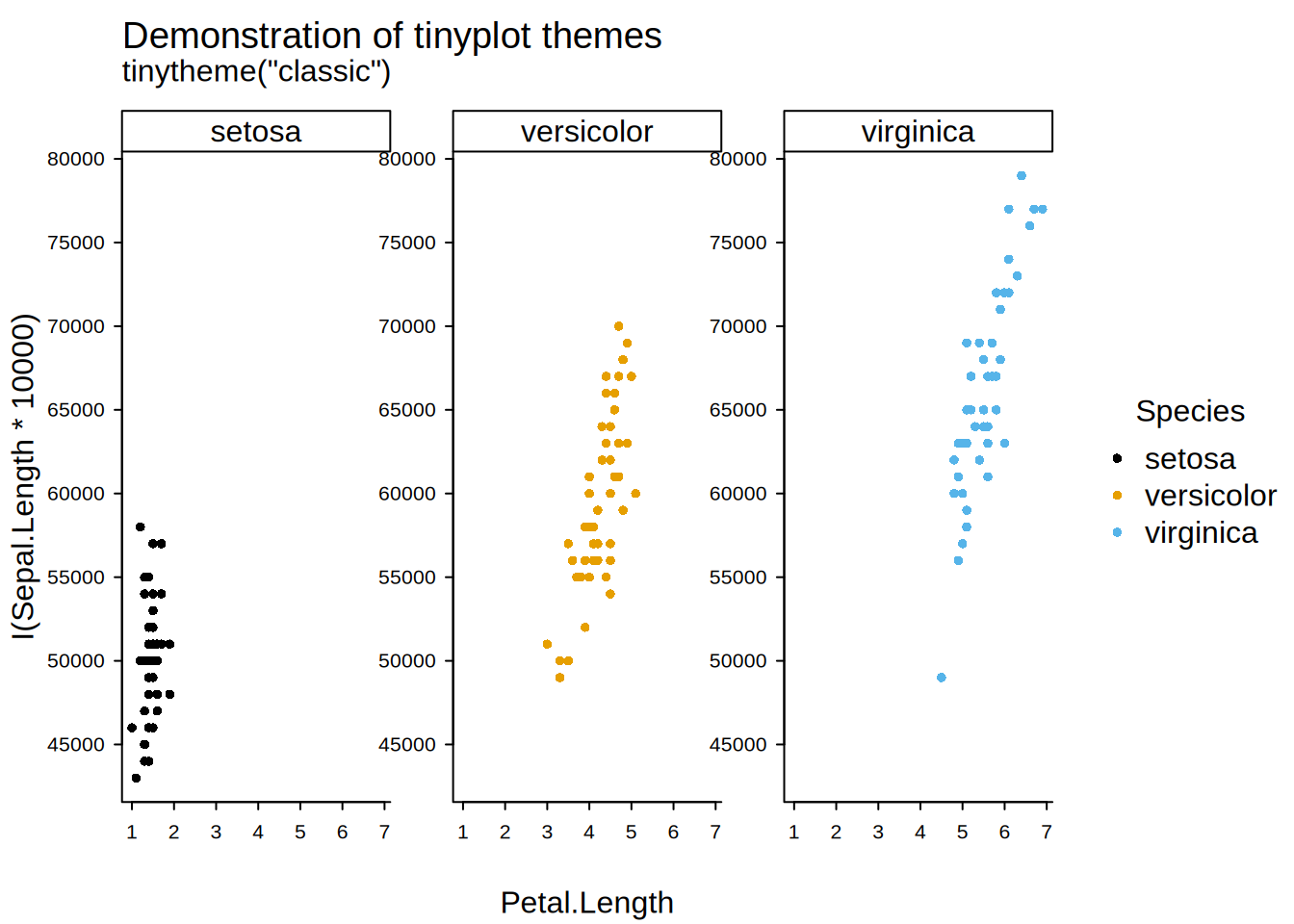“classic” (*): builds on “dynamic” with L-shaped axes (removing the top and right-hand edges of the plot frame), smaller axis text, tighter axis spacing, and the "Okabe-Ito" palette as a default for discrete colors. Inspired by the ggplot2 theme of the same name. 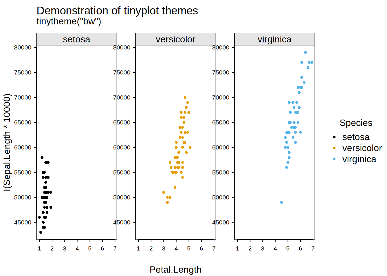“bw” (*): similar to “clean”, except uses thinner lines for the plot frame (box), solid fine grid lines, smaller axis text, tighter axis spacing, and sets the "Okabe-Ito" palette as a default for discrete colors. Inspired by the ggplot2 theme of the same name. “linedraw” (*): builds on “bw” with black facet title strips and white strip text. Inspired by the ggplot2 theme of the same name. 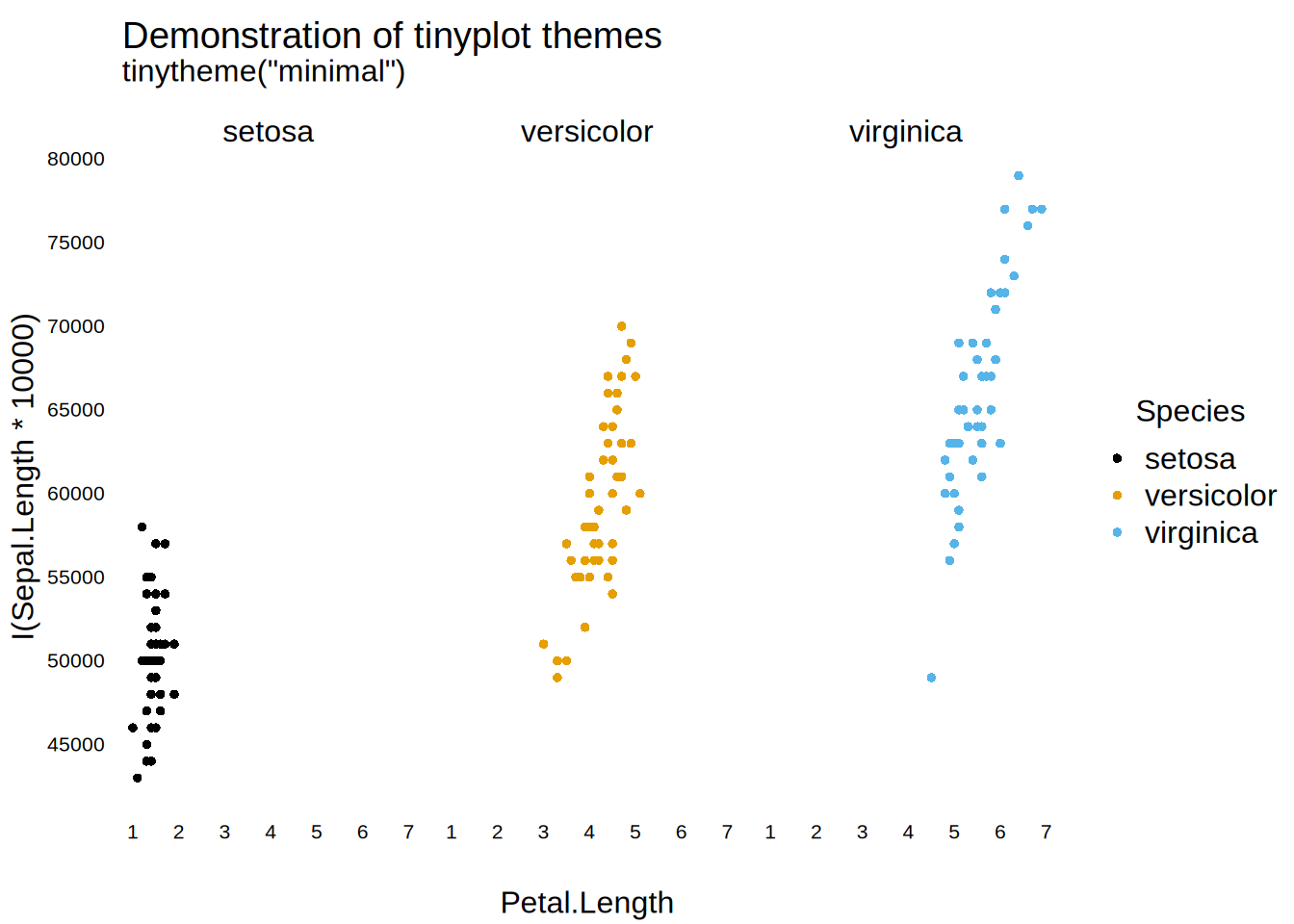“minimal” (*): removes the plot frame (box) from “bw”, as well as the background for facet titles. Inspired by the ggplot2 theme of the same name. 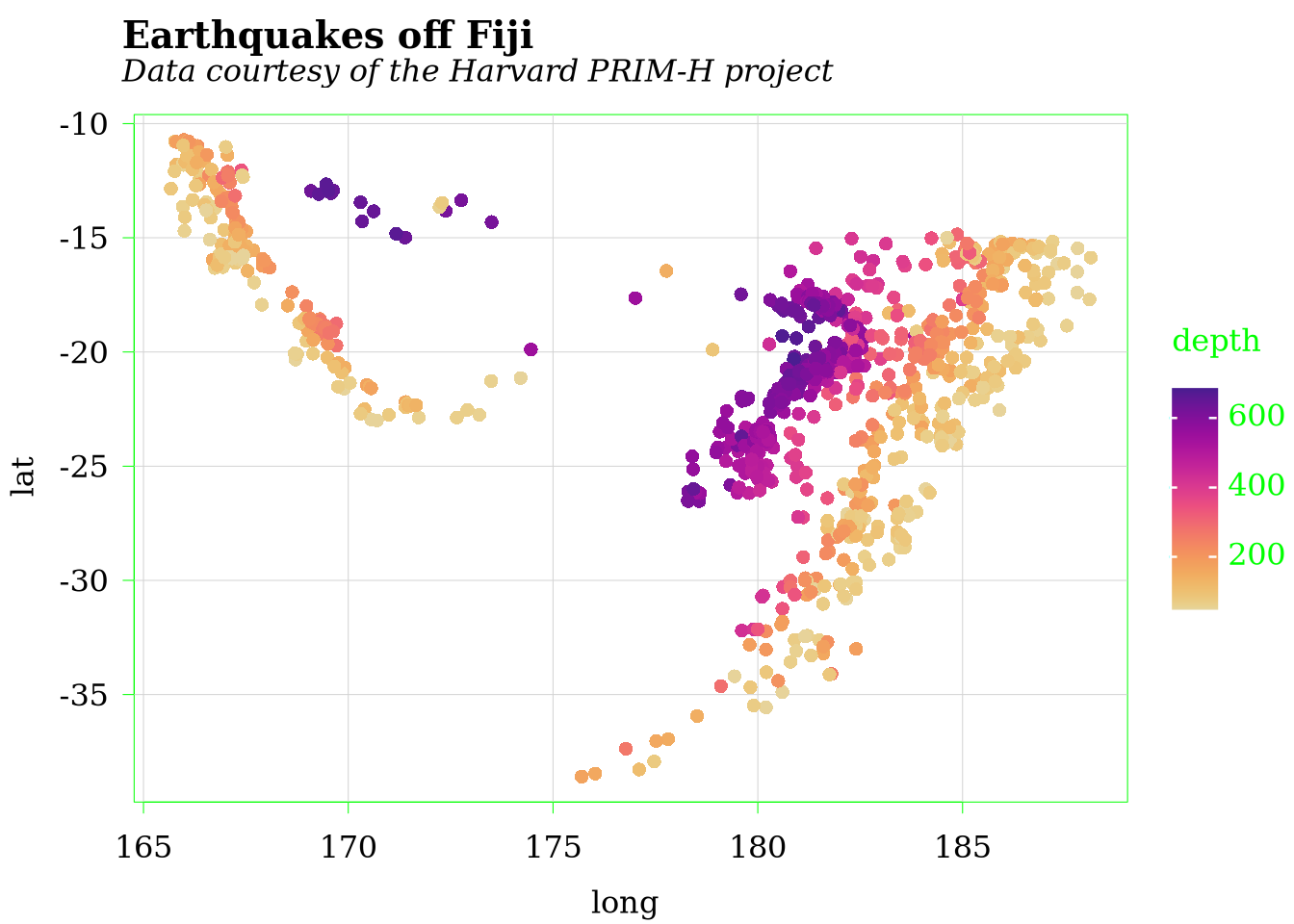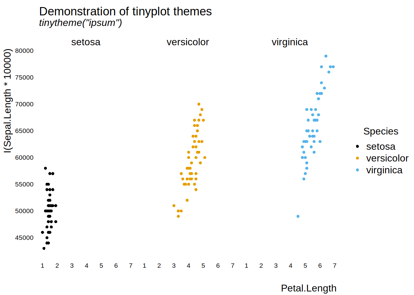“ipsum” (*): builds on “minimal” with bold titles, no ticks, fine grid, edge-aligned axis titles, and a custom muted palette. Inspired by the hrbrthemes theme of the same name for ggplot2. 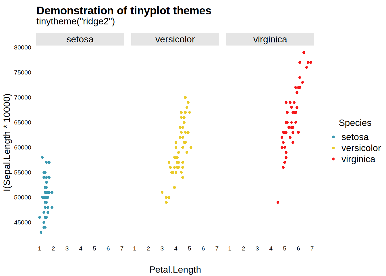“ipsum2” (*): a lighter variant of “ipsum” that retains the original italic subtitle and edge-aligned axis titles, but without the additional spacing and palette changes. 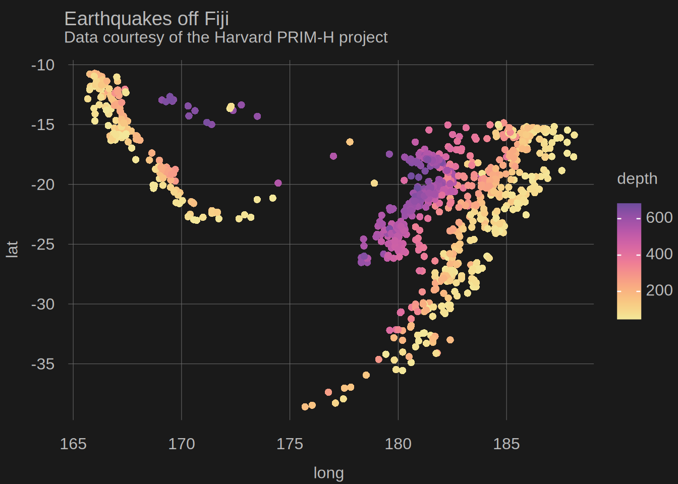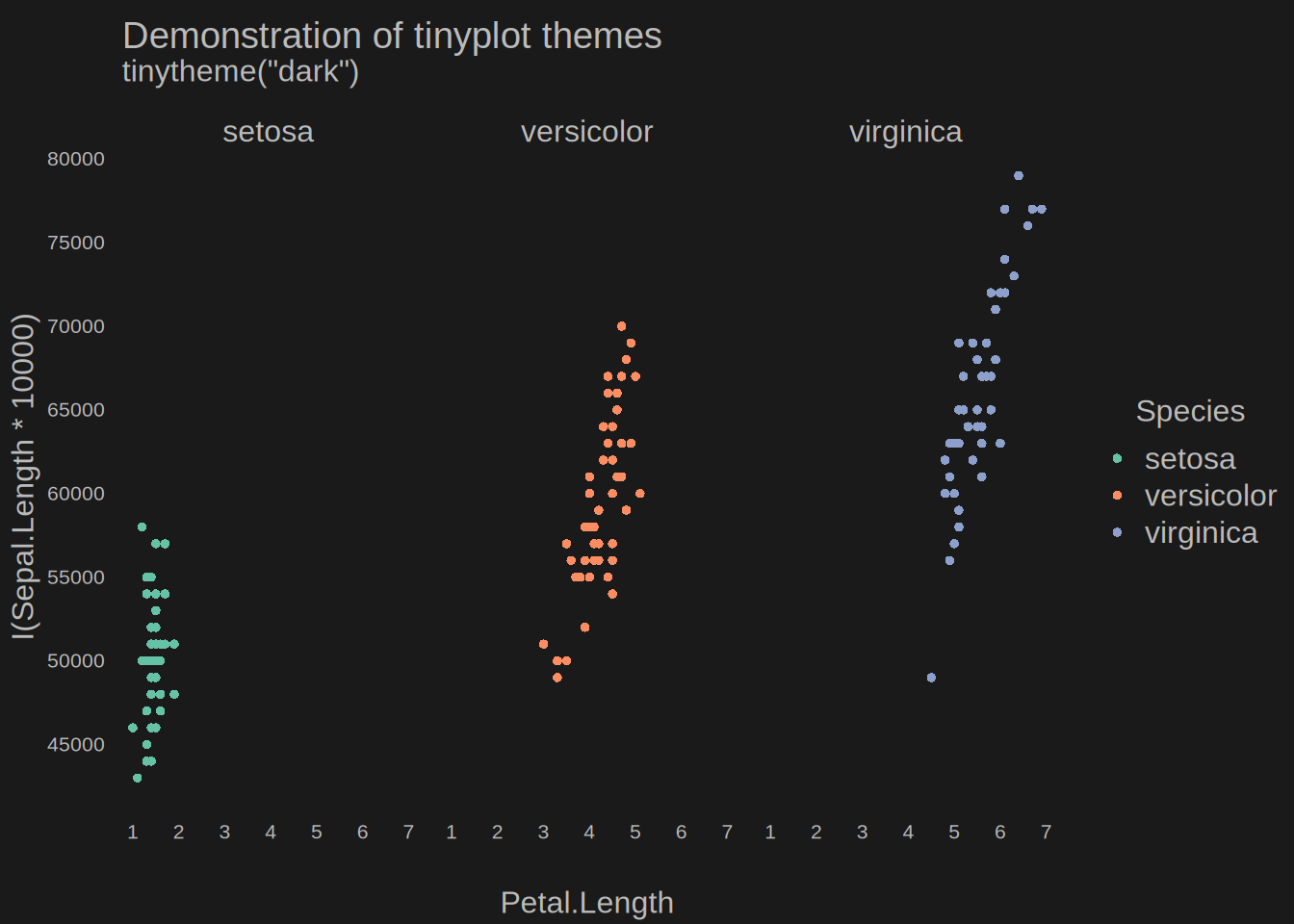“dark” (*): similar to “minimal”, but set against a dark background with foreground and a palette colours lightened for appropriate contrast. “socviz” (*): builds on “minimal” with L-shaped axes, very light grid lines, and larger axis text. Inspired by Kieran Healy’s socviz package theme for ggplot2. 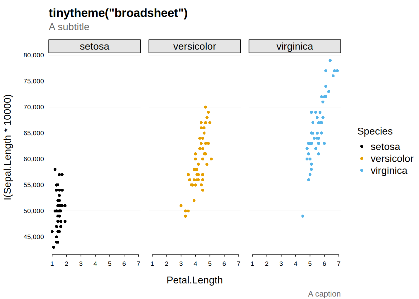“broadsheet” (*): a publication/newspaper style with only horizontal grid lines, no frame, short x-axis ticks, and muted secondary text (subtitle, caption). Compact axis spacing. 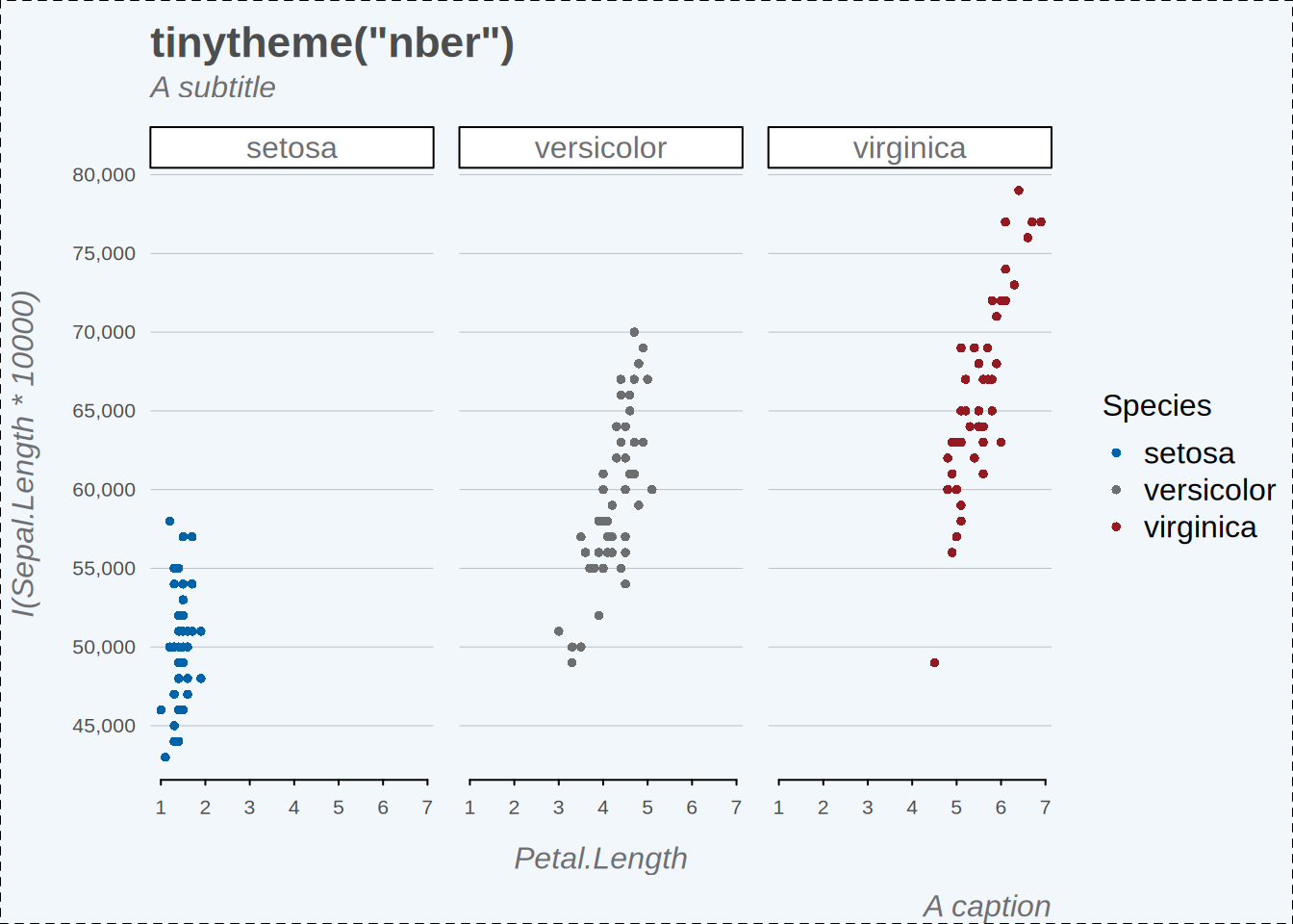“nber” (*): builds on “broadsheet” for an NBER working paper style with a light blue-grey background, grey text, italic axis titles and captions, and a blue-grey discrete palette. 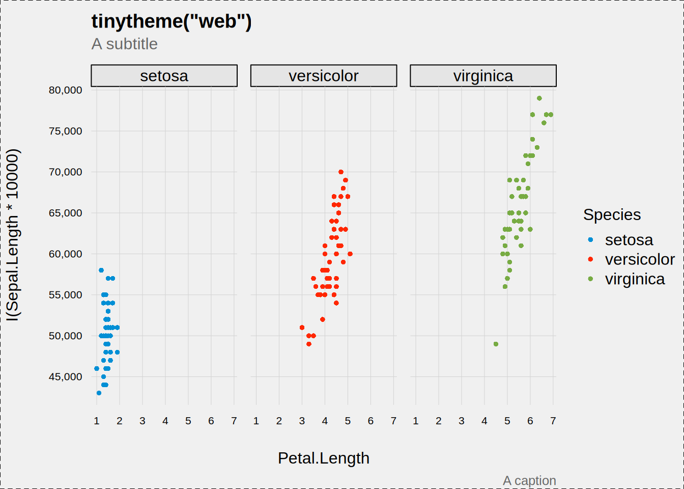“web” (*): a FiveThirtyEight-inspired style with a light grey device background, no frame or axis lines, and bold grid lines. Suited to web/online publication. 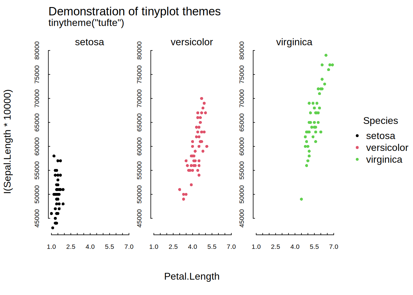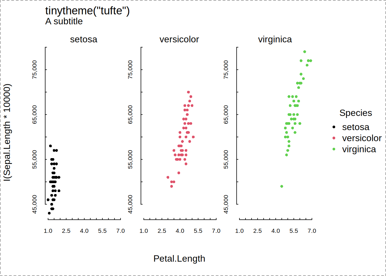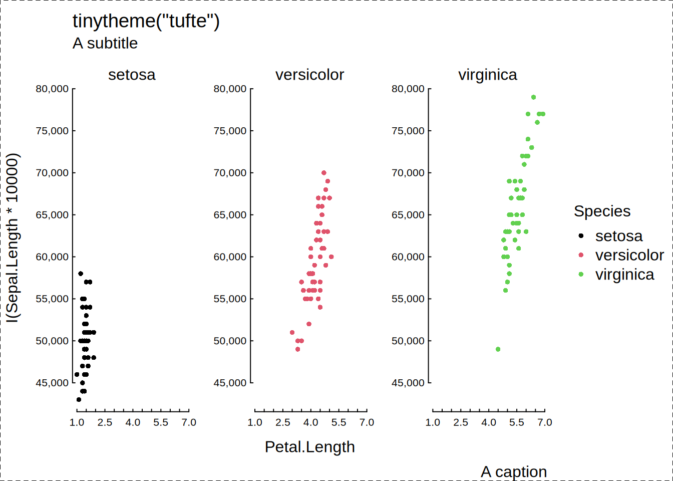“tufte” (*): floating axes and minimalist plot artifacts in the style of Edward Tufte. “float” (*): builds on “tufte” with outward ticks, fewer tick marks, and a "dark" qualitative palette. 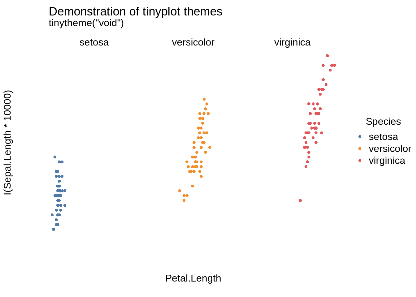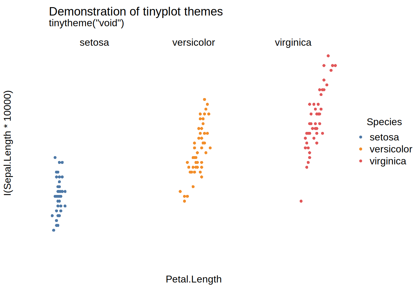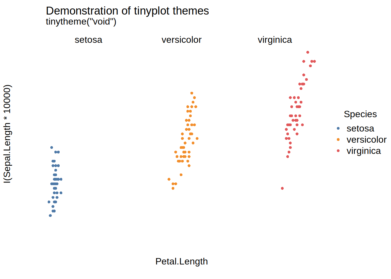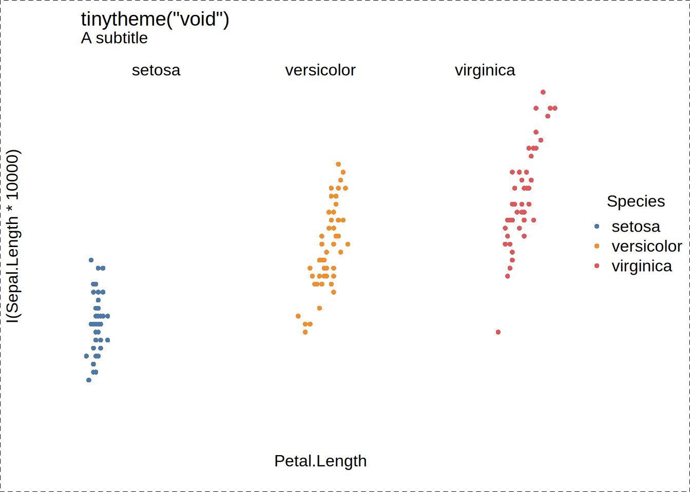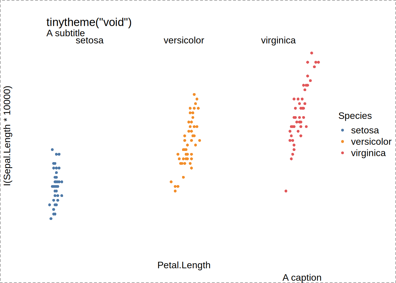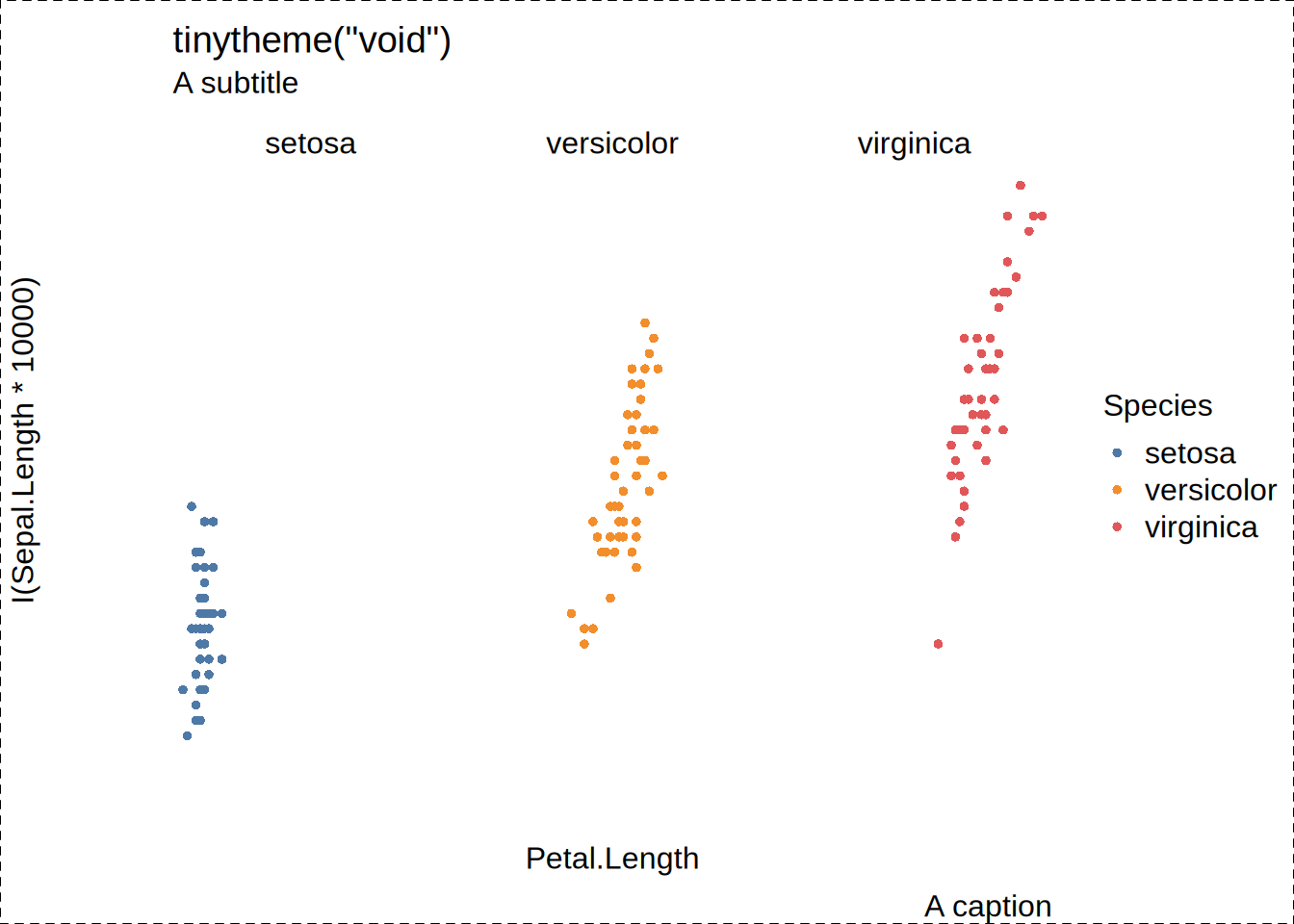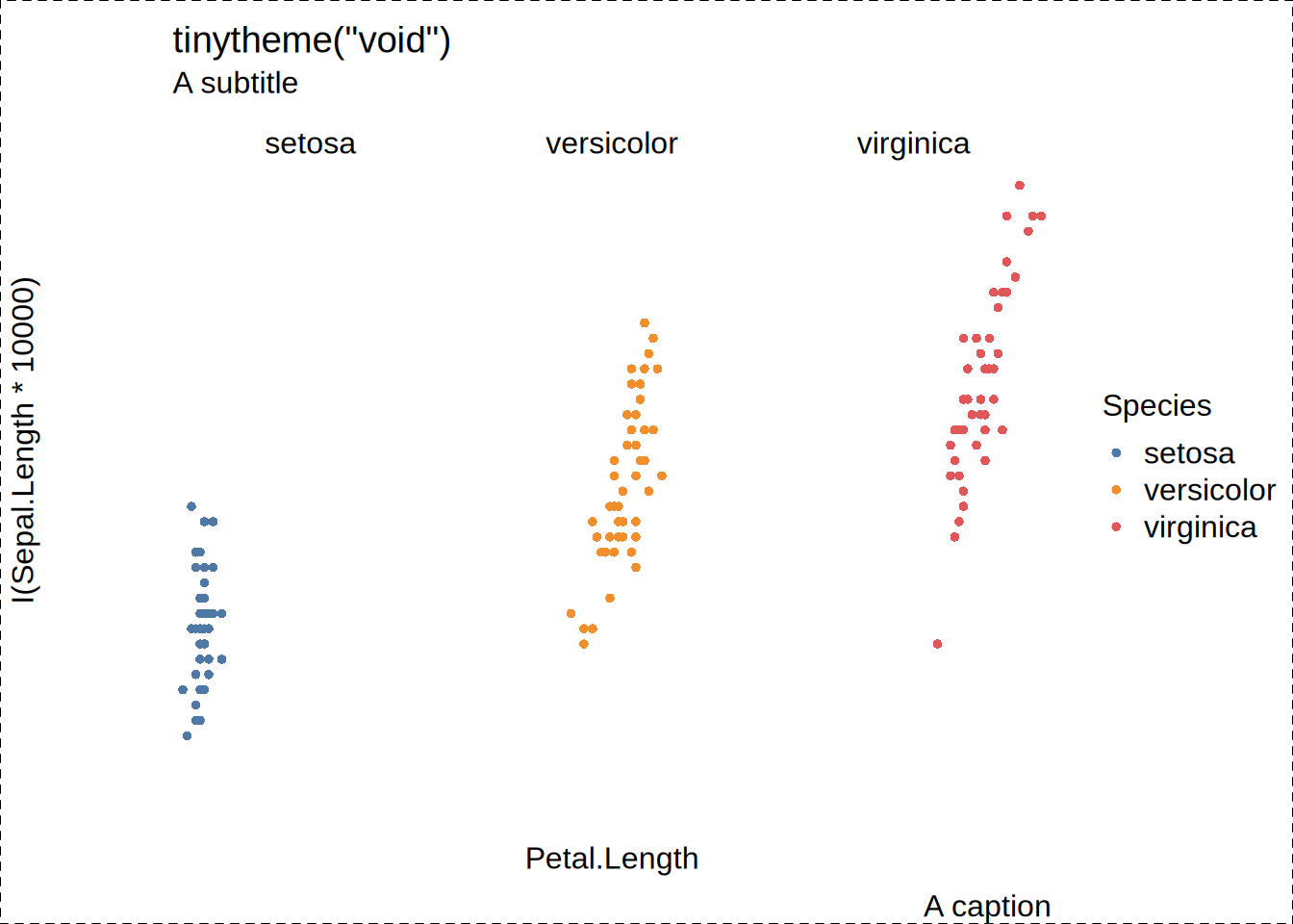“void” (*): switches off all axes, titles, legends, etc. “heatmap” (*): a specialized theme for tile plots and heatmaps (see type_tile()). Builds off of “clean2”, but removes the axis padding so that the tiles meet the panel edge, drops the (redundant) grid lines, rotates the tick labels and removes their tick marks, and defaults to the "tealgrn" sequential palette. Not recommended for non-tile plots. 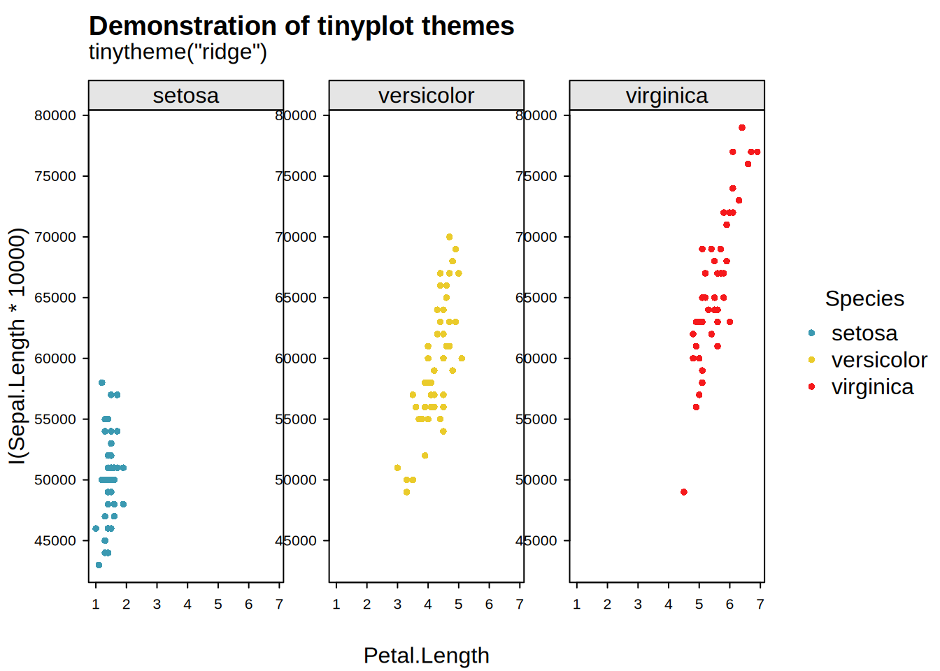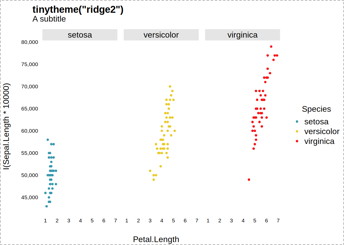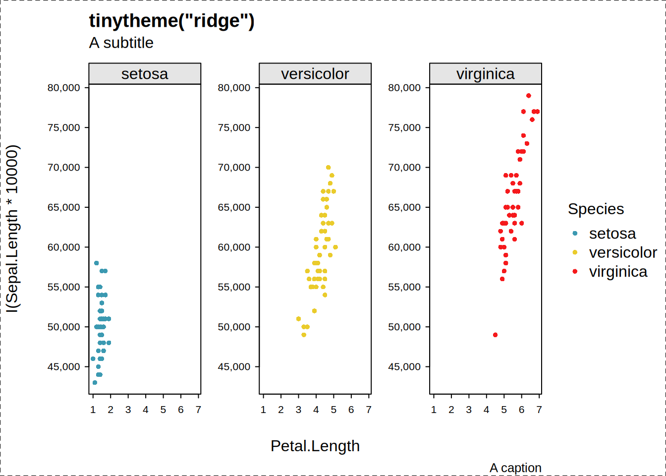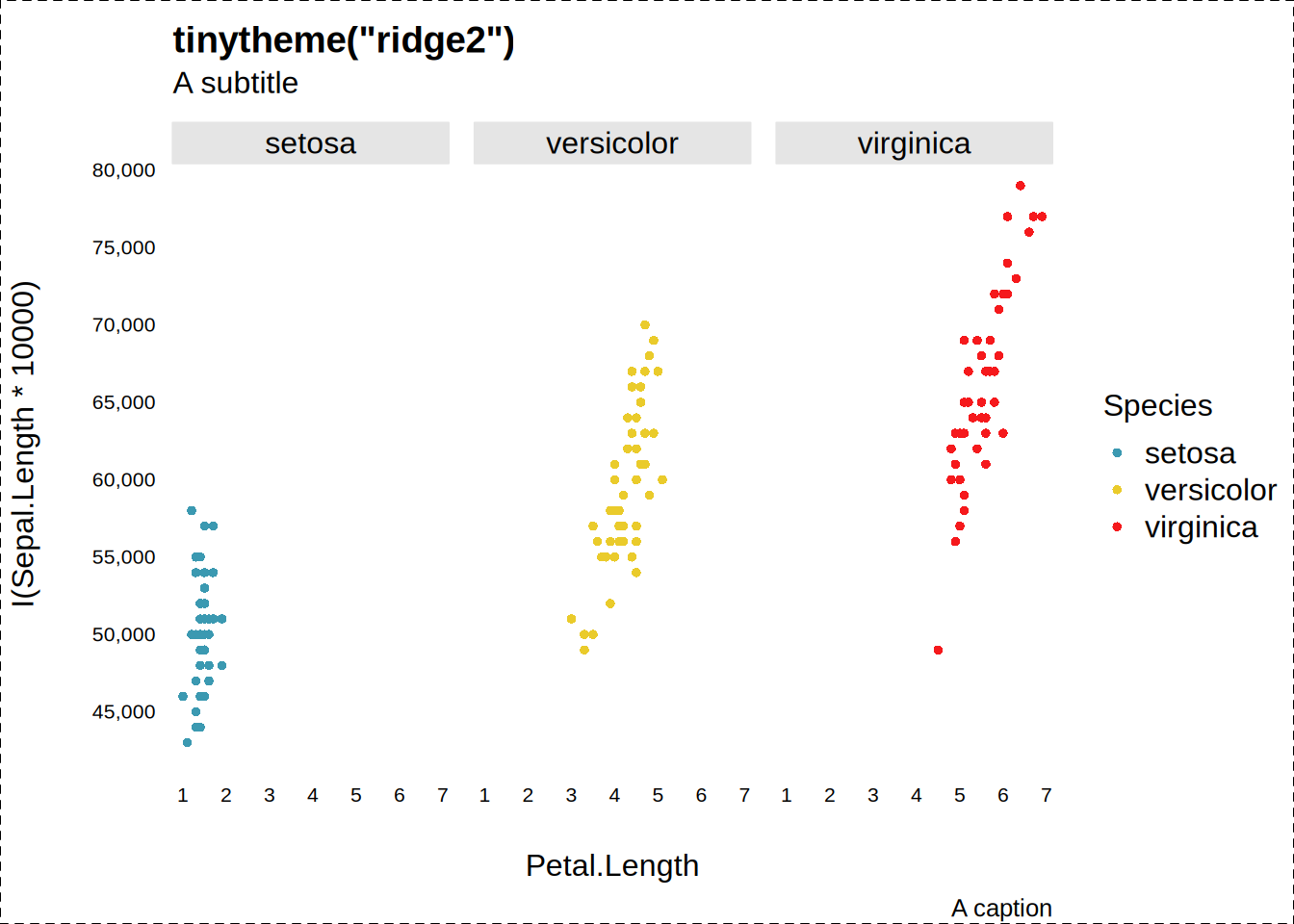“ridge” (*): a specialized theme for ridge plots (see type_ridge()). Builds off of “clean”, but adds ridge-specific tweaks (e.g. default "Zissou 1" palette for discrete colors, solid horizontal grid lines, and minor adjustments to y-axis labels). Not recommended for non-ridge plots. “ridge2” (*): removes the plot frame (box) from “ridge”, but retains the x-axis line. Again, not recommended for non-ridge plots.
…	Named arguments to override specific theme settings. These arguments are passed to tpar() and take precedence over the predefined settings in the selected theme.
register	Optional character string. If provided, the theme (with any … overrides) is registered under this name via tinytheme_register() and simultaneously activated. This is a shortcut for calling tinytheme_register() and tinytheme() separately.

Details

Sets a list of graphical parameters using tpar()

Persistent vs. ephemeral themes. Calling tinytheme(“<theme>”) triggers a persistent theme, which will be applied to all subsequent graphics (incl. base plot). To reset the theme to your default settings, call tinytheme() without arguments. Alternatively, invoke the tinyplot(…, theme = <theme>) argument for an ephemeral theme that is automatically reset at the end of the plot call.

# Set a persistent theme
tinytheme("clean")
tinyplot(1:10)  # uses "clean"
tinyplot(10:1)  # still uses "clean"
tinytheme()     # reset to default

# Use an ephemeral theme for a single plot (incl. added components)
tinyplot(1:10, theme = "dark")  # uses "dark" ephemerally
tinyplot_add(type = "S")        # same plot, so retains theme
tinyplot(10:1)                  # new plot, so back to default

Custom overrides. To customize a theme’s parameters (e.g., mar, las, etc.), either pass them directly as additional args to tinytheme(<theme>, …) or as a list arguments to tinyplot(…, theme = list(<theme>, …)). Please note that passing overrides through tpar() or par() won’t work, because themes work by installing a persistent hook, which means that an active theme will override any subsequent calls for parameters that the theme controls.

# Do this
tinytheme("clean", mar = c(5, 5, 2, 2))
<some plot>

# Or this (ephemeral version)
tinyplot(..., theme = list("clean", mar = c(5, 5, 2, 2)))

# Don't do this (the theme hook will overwrite your changes)
tinytheme("clean")
tpar(mar = c(5, 5, 2, 2))
<some plot>

Spacing primitives. Dynamic themes compute mgp (margin line positions) automatically from two spacing primitives, rather than requiring users to reason about how mar, mgp, and tcl combine:

• gap.axis: the gap in margin lines between the tick tip and the near edge of the tick label. Default 0.2.

• gap.lab: the gap in margin lines between the far edge of the tick label and the near edge of the axis title. Default 1.0.

These primitives scale automatically with cex.axis and cex.lab, so the visible spacing between elements remains constant regardless of text size. To adjust spacing, pass them as overrides:

# Tighter spacing between tick labels and axis titles
tinytheme("clean", gap.lab = 0.5)

# More room between ticks and tick labels
tinytheme("clean", gap.axis = 0.5)

If you supply an explicit mgp value, it is used as-is and the primitives are ignored.

Value

The function returns nothing. It is called for its side effects.

See Also

tpar which does the heavy lifting under the hood; tinytheme_register() for registering custom named themes.

Examples

library("tinyplot")

# Reusable plot function
p = function() tinyplot(
  lat ~ long | depth, data = quakes,
  main = "Earthquakes off Fiji",
  sub = "Data courtesy of the Harvard PRIM-H project"
)
p()

# Set a theme
tinytheme("dark")
p()

#  A set theme is persistent and will apply to subsequent plots
tinyplot(0:10)

# Try a different theme
tinytheme("clean")
p()

# Customize the theme by overriding default settings
tinytheme("clean",
          adj.xlab = 1, adj.ylab = 1,
          cex.lab = 0.75, cex.axis = 0.9,
          font.sub = 3,
          gap.axis = 0, gap.lab = 0.5,
          tcl = -0.1)
p()

# Another custom theme example, including a different font
tinytheme("bw", font.main = 2, col.axis = "darkcyan", family = "HersheyScript")
p()

# Aside: One or two specialized themes are only meant for certain plot types
tinytheme("ridge2")
tinyplot(I(cut(lat, 10)) ~ depth, data = quakes, type = "ridge")

# Reset the theme
tinytheme()
p()

# For an ephemeral theme, use `tinyplot(..., theme = <theme>)` directly
tinyplot(0:10, theme = "clean", main = "This theme is ephemeral")

tinyplot(10:0, main = "See, no more theme")

# Customize an ephemeral theme by passing arguments as a list
tinyplot(0:10, main = "Custom", theme = list("clean", grid.col = "hotpink"))

# Themes showcase
## We'll use a slightly more intricate plot (long y-axis labs and facets)
## to demonstrate dynamic margin adjustment etc.

thms = eval(formals(tinytheme)$theme)

for (thm in thms) {
  tinytheme(thm)
  tinyplot(
    I(Sepal.Length*1e4) ~ Petal.Length | Species, facet = "by", data = iris,
    yaxl = ",", 
    main = paste0('tinytheme("', thm, '")'),
    sub = "A subtitle",
    cap = "A caption"
  )
  box("outer", lty = 2)
}

# Reset
tinytheme()