tinyplot Method for Plotting Arrays

Description

Convenience interface for visualizing array objects with tinyplot. Extends the tinyplot.matrix conventions to arrays with up to four dimensions, by mapping the higher dimensions to facets.

Usage

## S3 method for class 'array'
tinyplot(
  x,
  type = NULL,
  legend = NULL,
  facet = NULL,
  xlab = NULL,
  ylab = NULL,
  xy = NULL,
  ...
)

Arguments

x	an object of class “array”.
type	plot type passed on to tinyplot. Defaults to “p” (points).
legend	specification passed on to tinyplot. The default is to draw a legend when the matrix has named columns, and to suppress it otherwise. For “tile” and “heatmap” types it is suppressed by default.
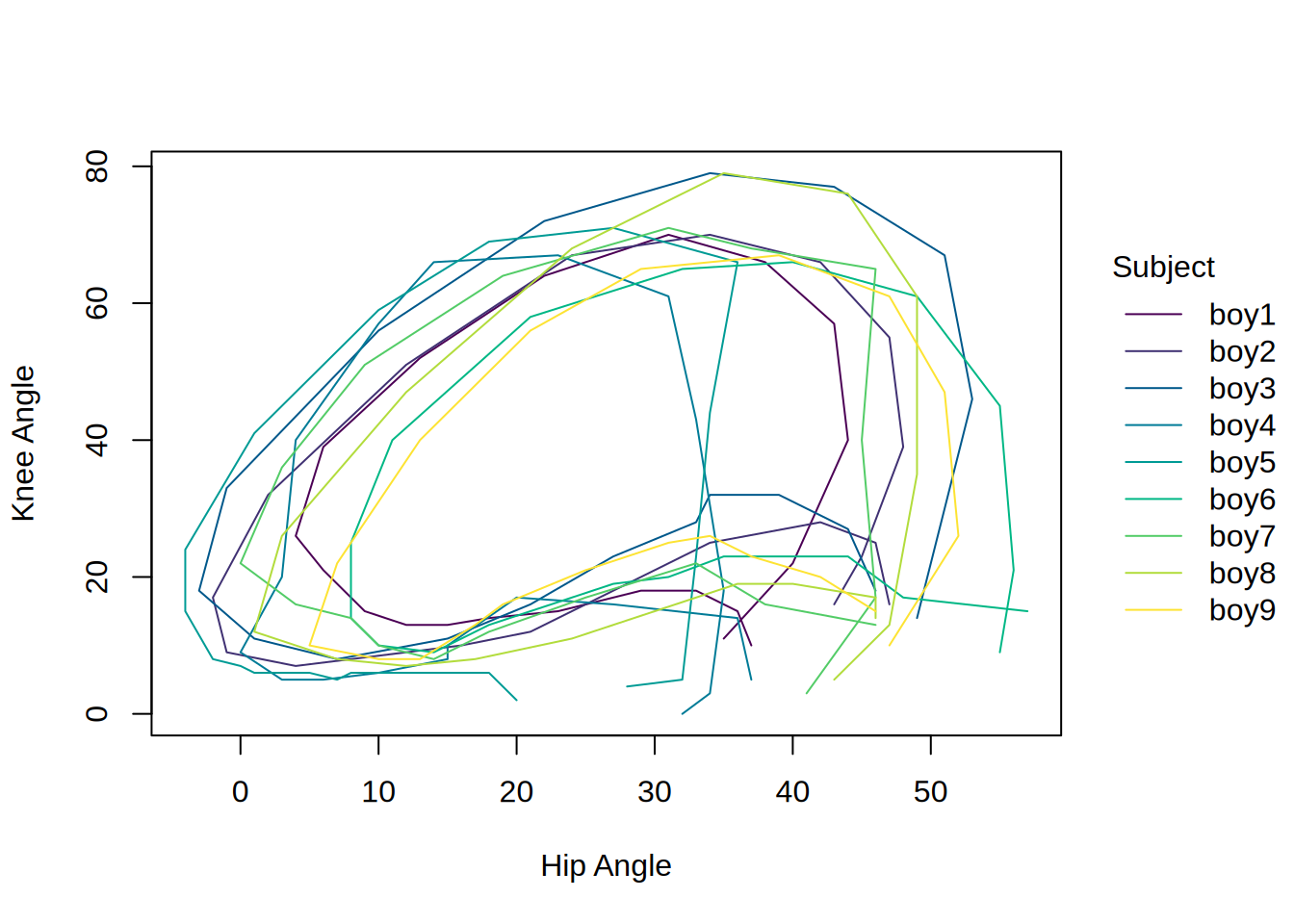
facet	must be NULL (the default) or FALSE for arrays with three or more dimensions, since the facets are then determined by the array dimensions. FALSE draws everything in a single panel instead, by folding the facet dimensions into the by groups. For x/y pairs, these groups then replace the first dimension as by, so that each path is drawn separately. Not supported for tile and heatmap types.
xlab, ylab	axis labels passed on to tinyplot. ylab defaults to the deparsed matrix name. xlab defaults to “Index” when the matrix has no row names; when it does, the row names already label the ticks so the x-axis title is suppressed. For “tile” and “heatmap” types both titles default to NA, since the dimnames label both axes.
xy	which dimension (if any) holds x/y pairs; see Details. The default NULL auto-detects it, FALSE opts out, and a dimension index or name selects it explicitly. The selected dimension must have length 2, and its dimnames (if any) are used as the axis titles.
…	further arguments passed to tinyplot.

Details

The first two dimensions of the array are treated exactly like the rows and columns of a matrix; see tinyplot.matrix. By default, that means the values are plotted against the (first dimension) row index, with a separate by group for each element of the second dimension. Higher dimensions are then mapped to facets:

• 1D arrays are treated as a single-column matrix, i.e. a simple index plot. If a y variable is also supplied, e.g. tinyplot(tapply(…), y), then the array is instead treated as a plain x vector.

• 2D arrays are matrices, and hence dispatch to tinyplot.matrix.

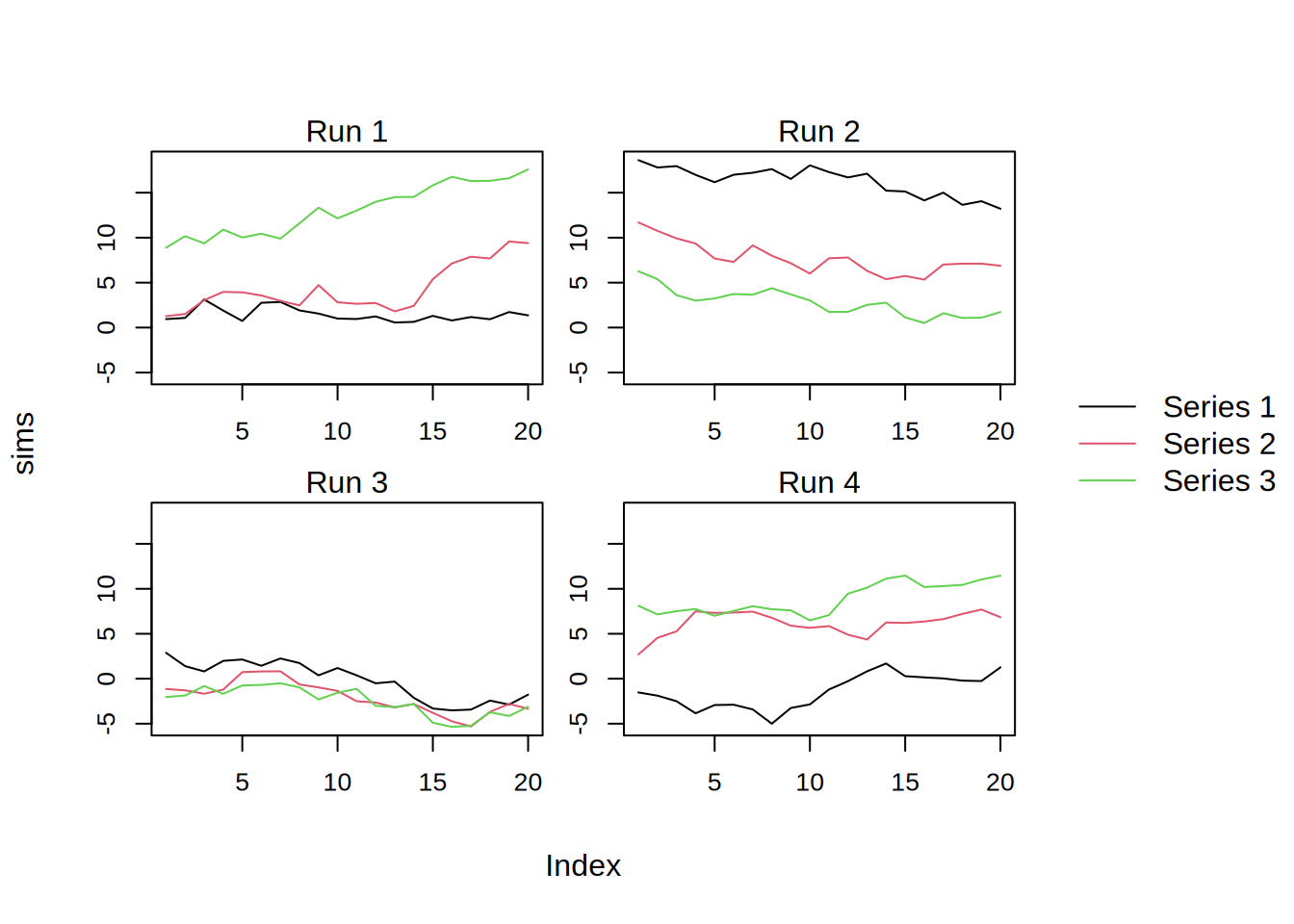
• 3D arrays are faceted by the third dimension (i.e., a "facet wrap").

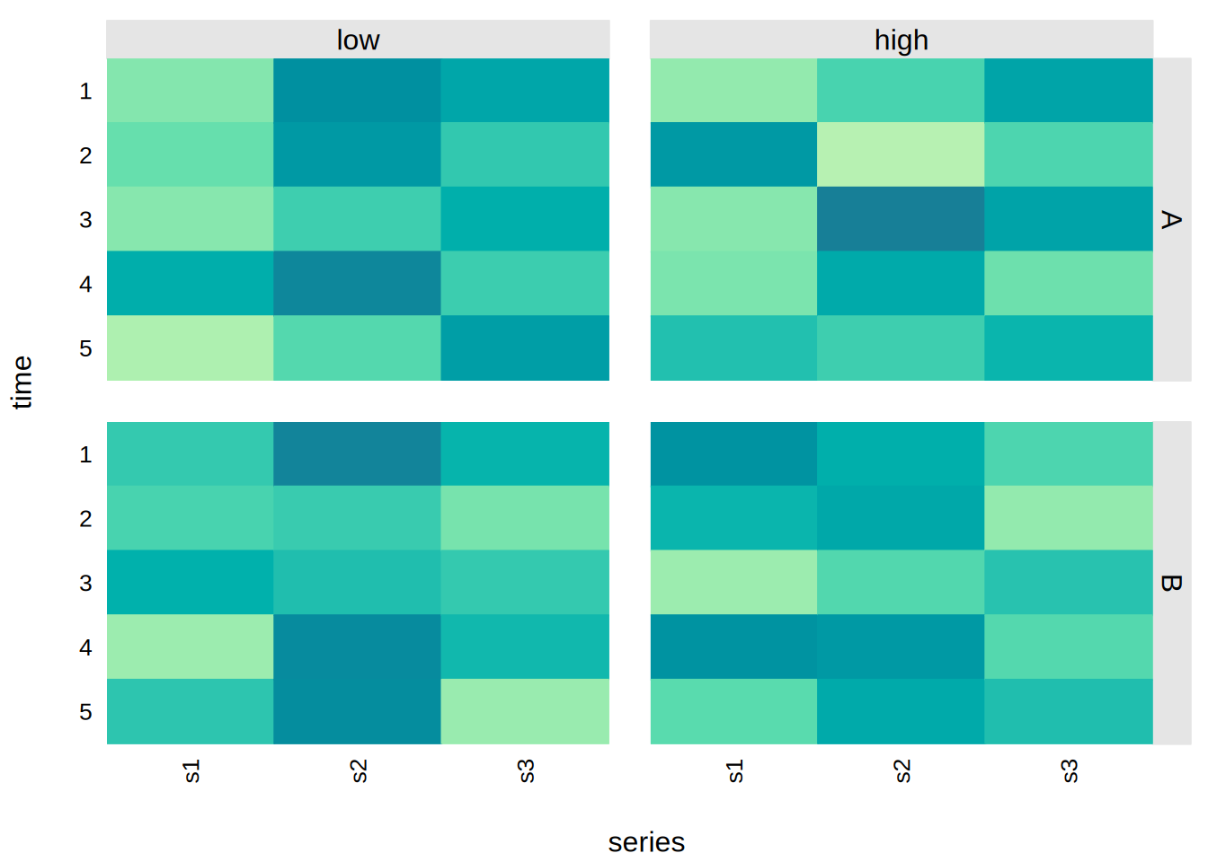
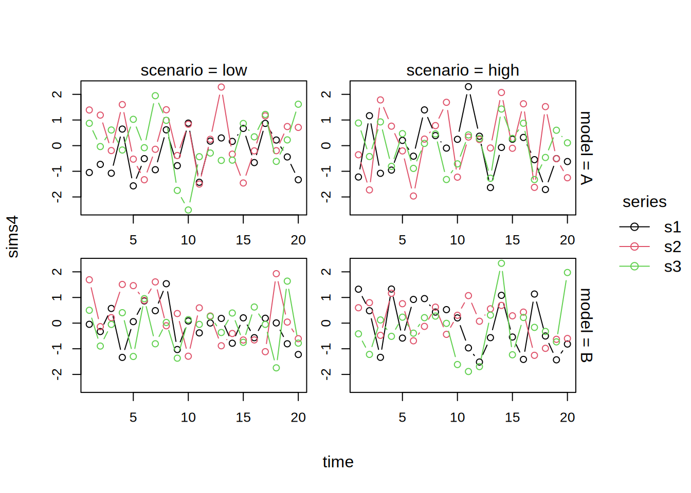
• 4D arrays are faceted by the third and fourth dimensions, as the rows and columns of a "facet grid", respectively.

• Arrays with more than four dimensions are not supported. Subset or reshape them first.

Dimension names are used to label the groups, facets, and axis ticks, while the names of the dimnames (if any) are used as the axis, legend, and facet titles. To assign the dimensions to different roles, rearrange them first with aperm.

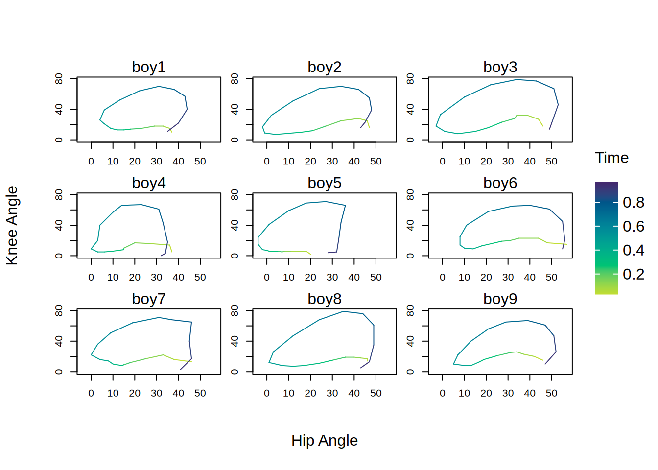
x/y pairs. Arrays often hold a stack of matrices, one per variable, e.g. the hip and knee angles of the gait data (Time x Subject x Variable). If an array of three or more dimensions has exactly one length-2 dimension besides the first, then its two slices are plotted against each other, as x and y. Each of the remaining dimensions then shifts down a role:

• The first dimension becomes by, and orders the points along each path. It is kept numeric where possible (its dimnames, e.g. times, or else its index), so that each path is drawn as a line with a colour gradient. If the dimnames are not numeric, then the groups are discrete and drawn as points instead.

• The second dimension becomes a facet wrap (e.g. one panel per subject).

• The third dimension (if any) makes this a facet grid, as its columns.

Control this via the xy argument. Tile and heatmap types are exempt, since they need the array values as their fill.

Note that contingency tables created by table (e.g., HairEyeColor or Titanic) are of class “table” and hence do not dispatch to this method.

Value

By default, no return value; called for the side effect of producing a plot. If record = TRUE (or globally via tpar(record = TRUE)), the plot is instead returned invisibly as a “recordedtinyplot” object, which can be replayed later; see recordedtinyplot.

See Also

tinyplot.matrix, matplot

Examples

library("tinyplot")

# 3D array: facet wrap by the third dimension
sims = array(
  cumsum(rnorm(20 * 3 * 4)), dim = c(20, 3, 4),
  dimnames = list(NULL, paste("Series", 1:3), paste("Run", 1:4))
)
tinyplot(sims, type = "l")

# 4D array: facet grid by the third and fourth dimensions
sims4 = array(
  rnorm(20 * 3 * 2 * 2), dim = c(20, 3, 2, 2),
  dimnames = list(
    time = NULL, series = paste0("s", 1:3),
    model = c("A", "B"), scenario = c("low", "high")
  )
)
tinyplot(sims4, type = "b", facet.args = list(prefix = TRUE))

# tile/heatmap types lay out each 2D slice as a grid
tinyplot(sims4[1:5, , , ], type = "heatmap", theme = "heatmap")

# x/y pairs: a length-2 dimension is plotted as x vs y
# (e.g., hip vs knee angle through the gait cycle, coloured by time and
# faceted by boy)
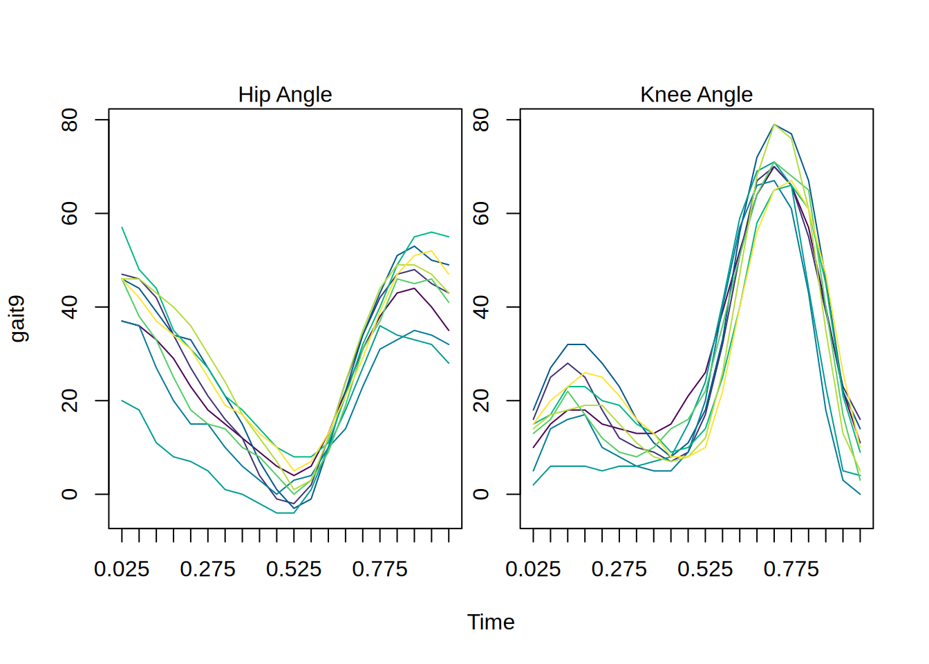
gait9 = gait[, 1:9, ] # take a subset for demonstration
tinyplot(gait9)

# all boys in a single panel instead
tinyplot(gait9, facet = FALSE)

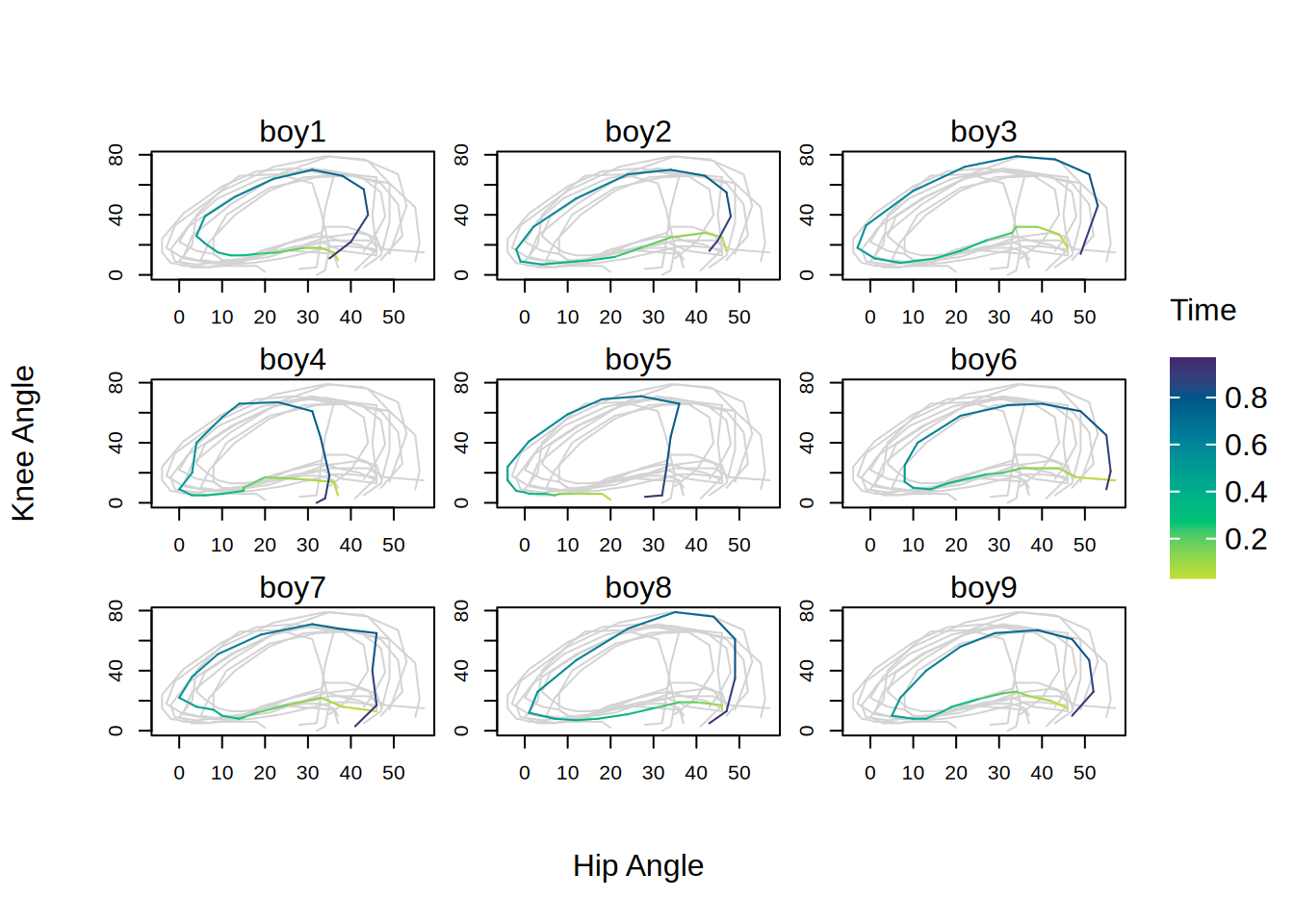
# ... or in the background of each boy's own panel
tinyplot(
  gait9,
  draw = tinyplot(gait9, col = "lightgray", facet = FALSE, add = TRUE)
)

# opt out of x/y pairs, to plot the angles against time instead
tinyplot(gait9, type = "l", xy = FALSE, legend = FALSE)