library(tinyplot)

aq = transform(
  airquality,
  Month = factor(Month, labels = month.abb[unique(Month)]),
  Hot = Temp > median(Temp)
)Plot types
tinyplot is a lightweight extension of R’s base plotting system, designed to simplify and enhance data visualization. One of its key features is the type argument, which allows you to specify different types of plots easily. This tutorial will guide you through the various plot types available in tinyplot, demonstrating how to use the type argument to create a wide range of visualizations.
We will consider three categories of plot types:
- Base types
tinyplottypes- Custom types
We will use the built-in airquality dataset for our examples:
Base types
The type argument in tinyplot supports all the standard plot types from base R’s plot function. These are specified using single-character strings.
The default plot type is "p", which creates a scatter plot of points.
tinyplot(Temp ~ Day | Month, data = aq, type = "p", main = "Points")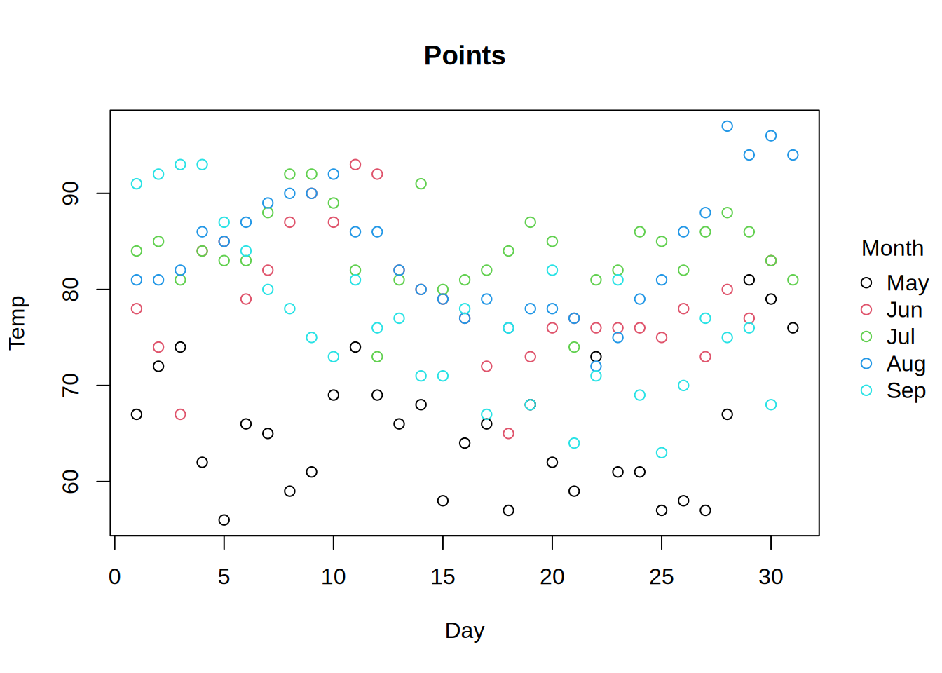
Use "l" to connect data points with lines.
tinyplot(Temp ~ Day | Month, data = aq, type = "l", main = "Lines")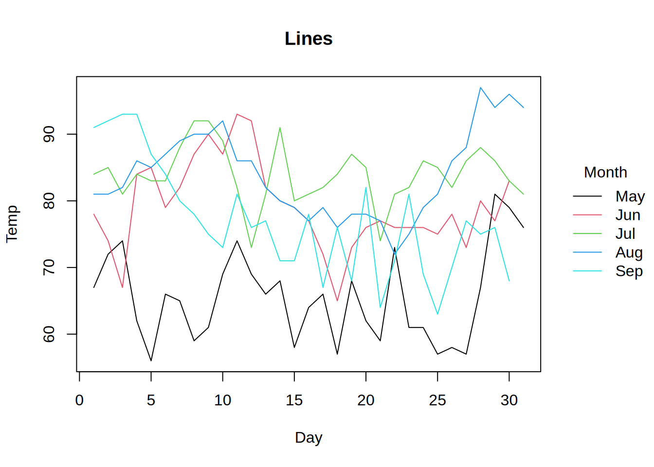
Other base plot types supported as single-character strings:
b(Points and Lines): Combines points and lines in the plot.c(Empty Points Joined by Lines): Plots empty points connected by lines.o(Overplotted Points and Lines): Overlaps points and lines.sandS(Stair Steps): Creates a step plot.h(Histogram-like Vertical Lines): Plots vertical lines resembling a histogram.n(Empty Plot): Creates an empty plot frame without data.
tinyplot types
Beyond the base types, tinyplot introduces additional plot types for more advanced visualizations.
Models:
loess,type_loess(): Local regression curve.lm,type_lm(): Linear regression line.glm,type_glm(): Generalized linear model fit.
Shapes:
segments: Draws line segments between pairs of points.polygon: Draws filled polygons.errorbar: Adds error bars to points; requires ymin and ymax.pointrange: Combines points with error bars.ribbon: Creates a filled area between ymin and ymax.area: Plots the area under the curve from y = 0 to y = f(x).rect: Draws rectangles; requiresxmin,xmax,ymin, andymax.
Visualizations:
jitter/type_jitter(): Jittered points.boxplot/type_boxplot(): Creates a box-and-whisker plot.histogram/type_histogram(): Creates a histogram of a single variable.density: Plots the density estimate of a variable.
There are two main ways to use tinyplot types. First, we can specify the type directly using a string shortcut in the type argument, such as type="boxplot".
Second, many tinyplot types are implemented by a type_*() function which includes arguments that allow us to customize the plot further. For example, the type_jitter() function includes arguments to control the amount of jittering, and the type_glm() includes an argument to control the width of the confidence interval to display. To see what arguments are available for each type, simply consult the type-specific documentation:
?type_jitter
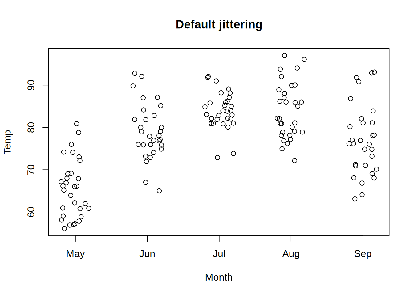
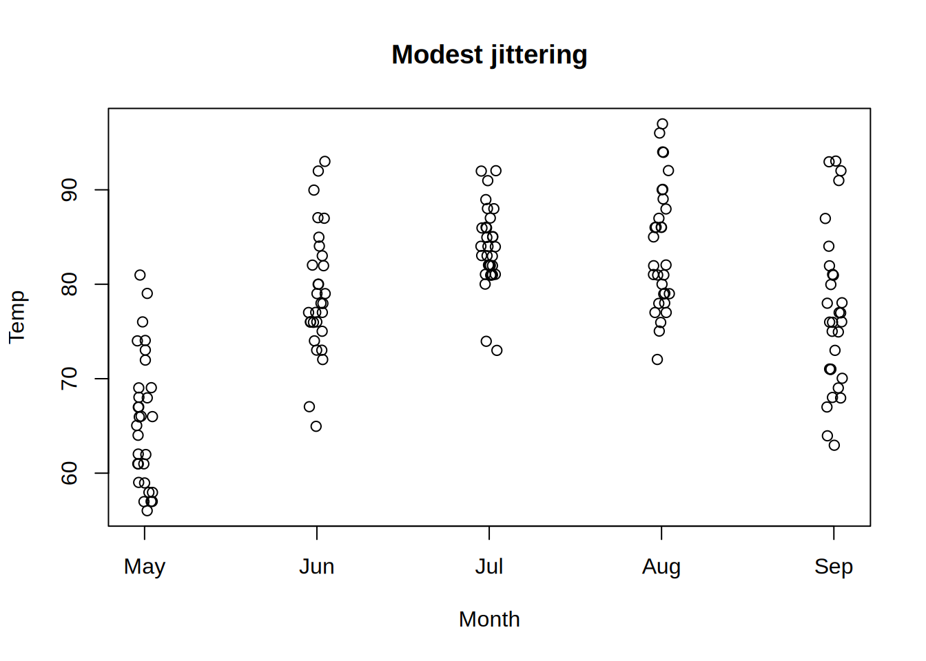
?type_glmFor example, we can add noise to data points using the "jitter" type. This allows us to avoid overplotting and can be useful to visualize discrete variables. On the left, we use the string shortcut with default settings. On the right, we use the type_jitter() function to select a smaller amount of jittering:
tinyplot(
  Temp ~ Month, data = aq, main = "Default jittering",
  type = "jitter"
)
tinyplot(
  Temp ~ Month, data = aq, main = "Modest jittering",
  type = type_jitter(amount = 0.05)
)
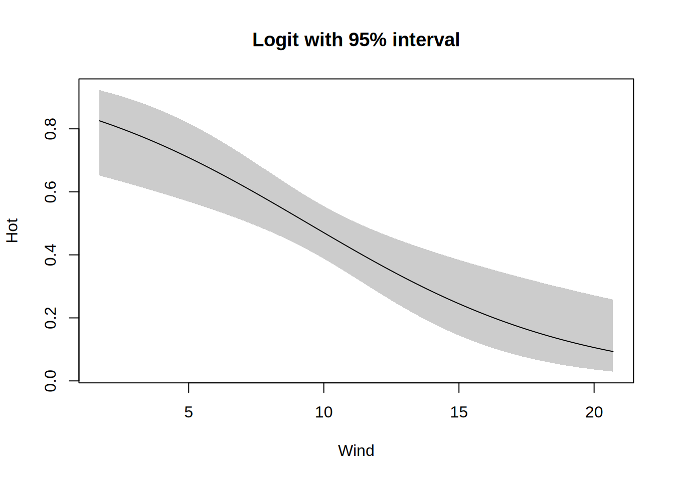
In this example, we use type_glm() to fit a logit regression model to the data, and display different confidence interval sizes:
tinyplot(
Hot ~ Wind, data = aq, main = "Logit with 95% interval",
type = type_glm(family = "binomial")
)
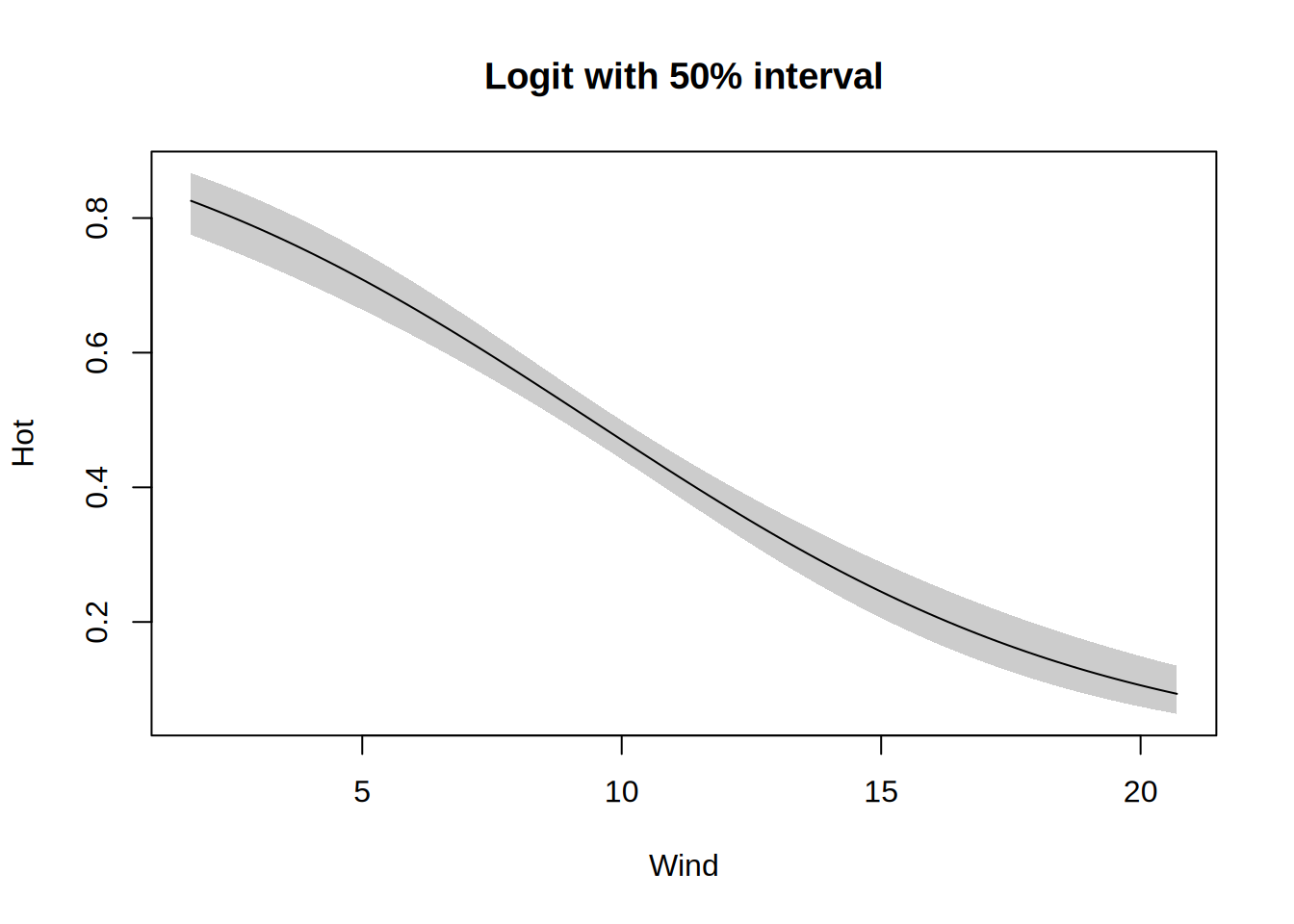
tinyplot(
Hot ~ Wind, data = aq, main = "Logit with 50% interval",
type = type_glm(family = "binomial", level = 0.5)
)
All tinyplot types should support grouping and faceting:
tinyplot(Temp ~ Wind | Month, data = aq, facet = "by", type = "lm")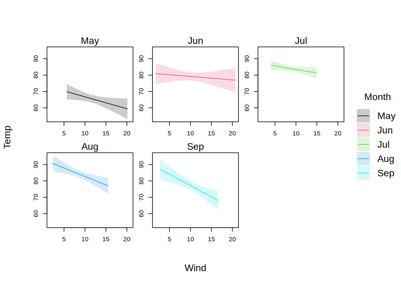
Custom types
It is easy to add custom types to tinyplot. Users who need highly customized plots, or developers who want to add support to their package or functions, only need to define three simple functions: data_typename(), draw_typename(), and type_typename().
In this section, we explain the role of each of these functions and present a minimalist example of a custom type. Interested readers may refer to the tinyplot source code to see many more examples, since each tinyplot type is itself implemented as a custom type.
The three functions that we need to define for a new type are:
data_*(): Function factory.- Accepts a list of internal objects
- Inputs must include
... datapointsIs the most important object. It is a data frame with the datapoints to plot.- Other objects that can be modified by
data_*()include:by,facet,ylab,palette
- Inputs must include
- Returns a named list with modified versions of those objects.
- Accepts a list of internal objects
draw_*(): Function factory.- Accepts information about data point values and aesthetics.
- Inputs must include
... - The
iprefix in argument names indicates that we are operating on a subgroup of the data, identified byfacetor using the|operator in a formula. - Available arguments are:
ibg,icol,ilty,ilwd,ipch,ix,ixmax,ixmin,iy,iymax,iymin,cex,dots,type,x_by,i,facet_by,by_data,facet_data,flip
- Inputs must include
- Returns a function which can call base R to draw the plot.
- Accepts information about data point values and aesthetics.
type_*(): A wrapper function that returns a named list with three elements:drawdataname
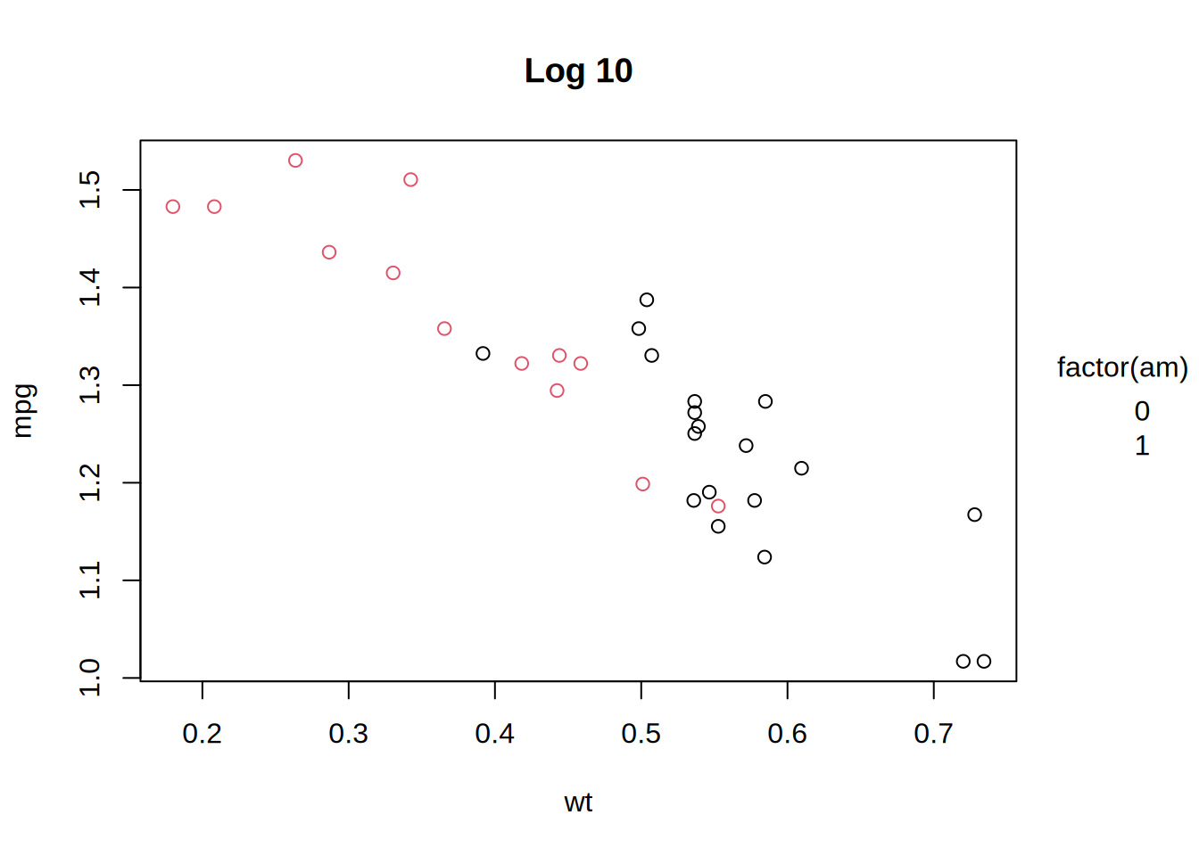
Here is a minimalist example of a custom type that logs both x and y and plots lines:
type_log = function(base = exp(1)) {

  data_log = function() {
    fun = function(datapoints, ...) {
      datapoints$x = log(datapoints$x, base = base)
      datapoints$y = log(datapoints$y, base = base)
      datapoints = datapoints[order(datapoints$x), ]
      return(list(datapoints = datapoints, ...))
    }
    return(fun)
  }

  draw_log = function() {
    fun = function(ix, iy, icol, ...) {
      points(
        x = ix,
        y = iy,
        col = icol
      )
    }
    return(fun)
  }

  out = list(
    draw = draw_log(),
    data = data_log(),
    name = "log"
  )
  class(out) = "tinyplot_type"
  return(out)
}

tinyplot(mpg ~ wt | factor(am), data = mtcars,
  type = "p", main = "Raw")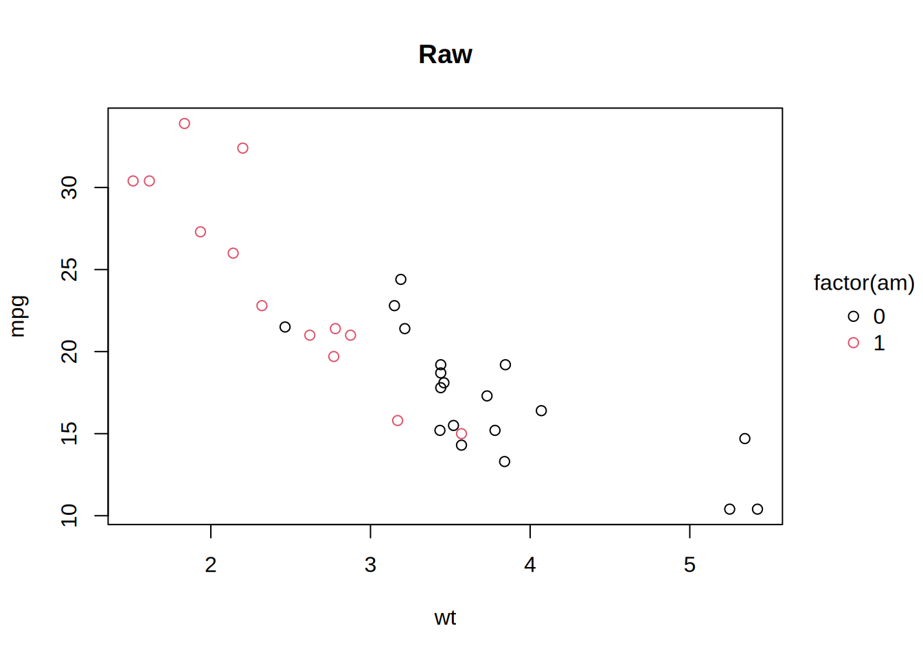
tinyplot(mpg ~ wt | factor(am), data = mtcars,
  type = type_log(), main = "Ln")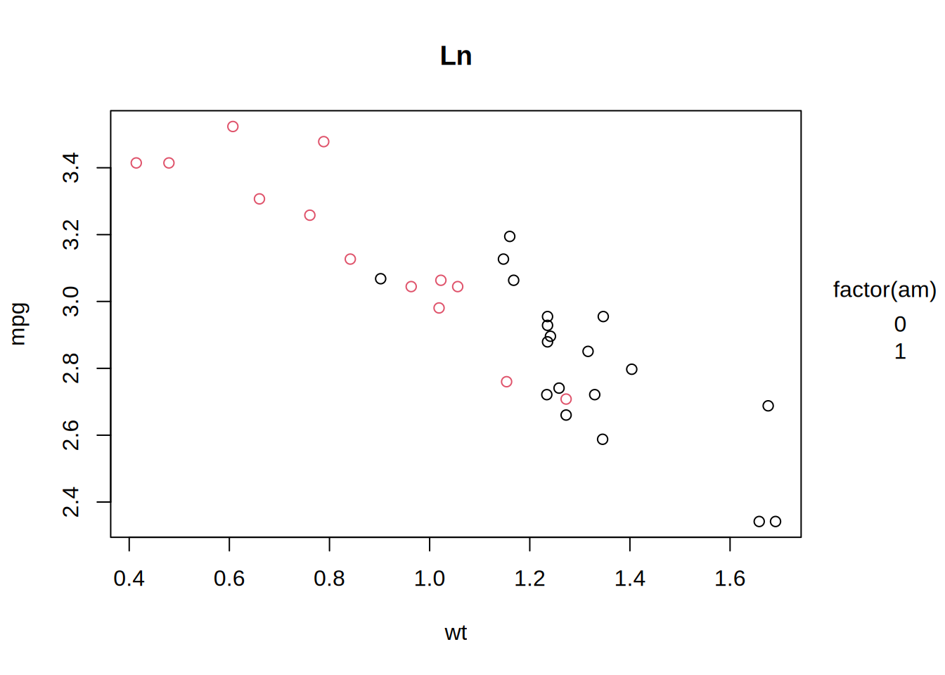
tinyplot(mpg ~ wt | factor(am), data = mtcars,
  type = type_log(base = 10), main = "Log 10")