plot.dbbinsreg

Plot method for dbbinsreg objects

Description

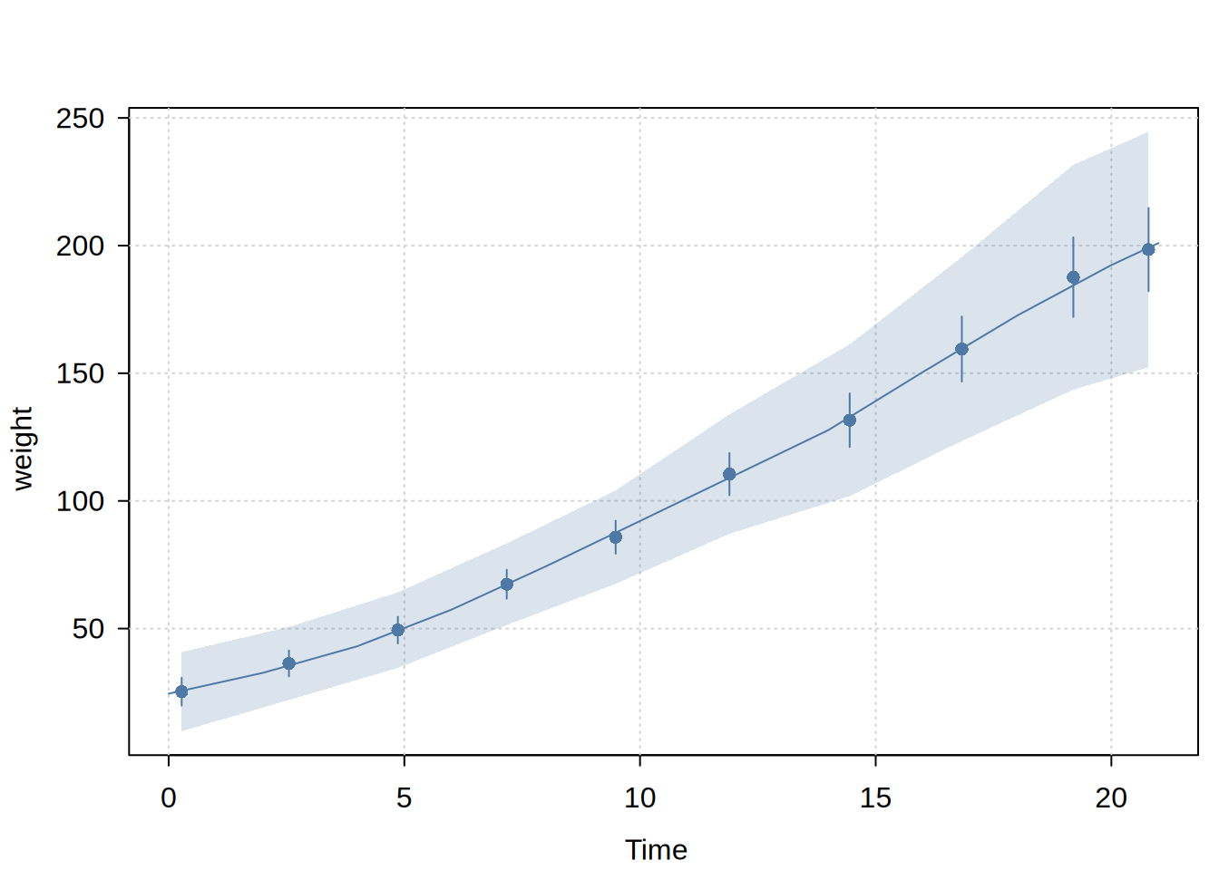
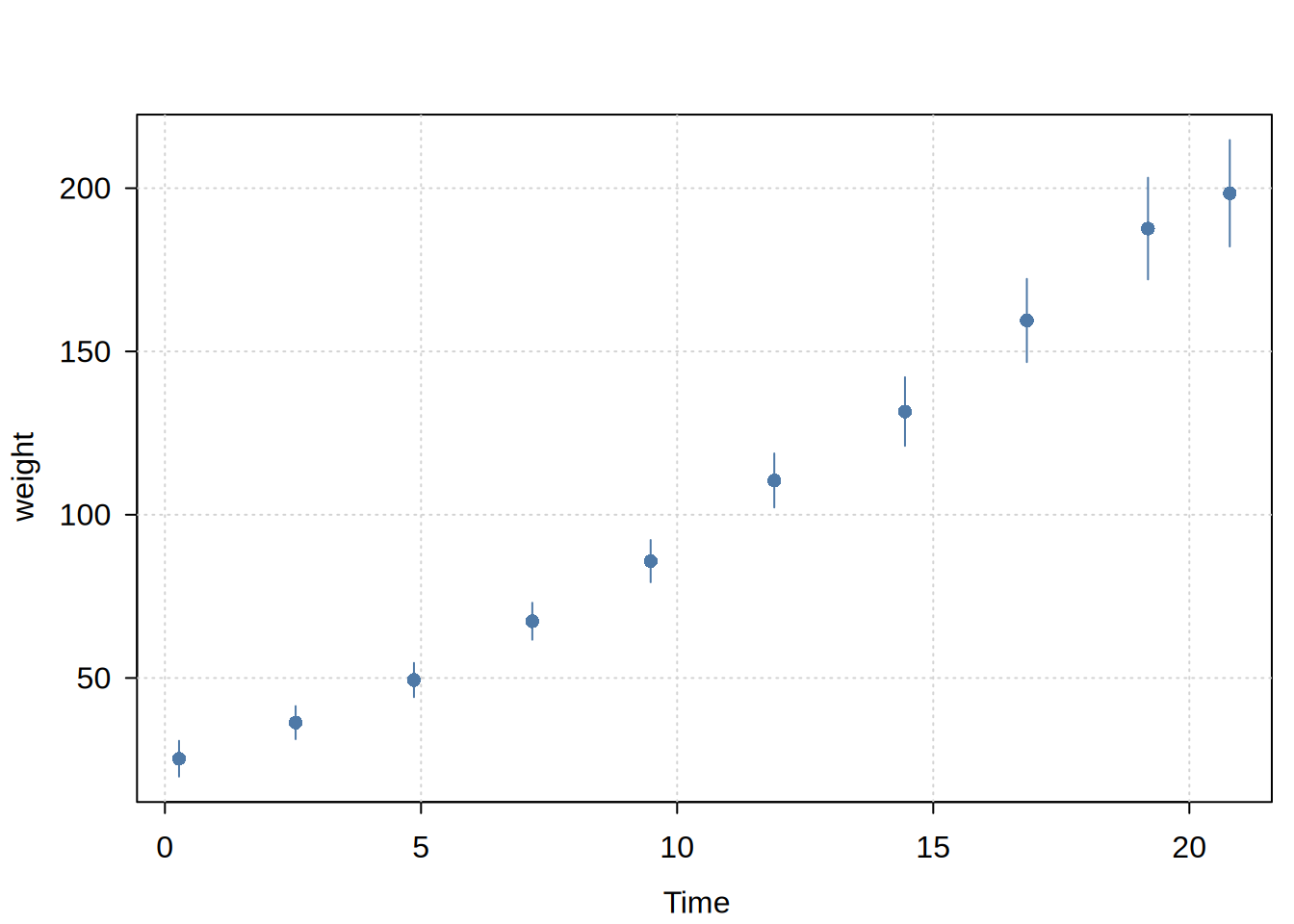
Visualizes binned regression results from dbbinsreg. Plots dots at bin means with optional confidence intervals and/or confidence bands, and optionally overlays a smooth line if computed. Uses tinyplot for rendering but works with both plot() and tinyplot() generics.

Usage

## S3 method for class 'dbbinsreg'
plot(
  x,
  type = NULL,
  ci = TRUE,
  cb = TRUE,
  line = TRUE,
  lty = 1,
  theme = "basic",
  ...
)

## S3 method for class 'dbbinsreg'
tinyplot(
  x,
  type = NULL,
  ci = TRUE,
  cb = TRUE,
  line = TRUE,
  lty = 1,
  theme = "basic",
  ...
)

Arguments

x A dbbinsreg object

type The type of plot. If NULL (the default), then the type will be inferred based on the underlying object (e.g, “pointrange” for points with confidence intervals).

ci Logical. Show confidence intervals for dots? Default is TRUE.

cb Logical. Show confidence bands as a ribbon? Default is TRUE if available in the object.

line Logical. Show the line overlay if available? Default is TRUE.

lty Integer or character string. Line type for line overlay.

theme Character string. One of the valid plot themes supported by tinytheme. The default “basic” theme is a light adaptation of the standard base graphics aesthetic, featuring filled points and a background grid. Various other themes are supported (e.g., “clean”, “minimal”, “classic”, etc.), while passing NULL switches the theme off entirely.

… Additional arguments passed to tinyplot, e.g. main, sub, file, etc.

Examples

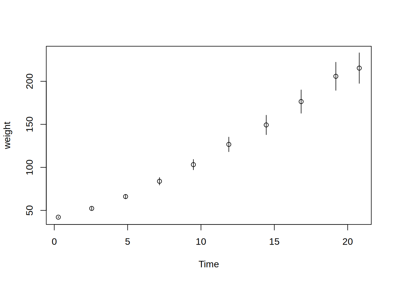
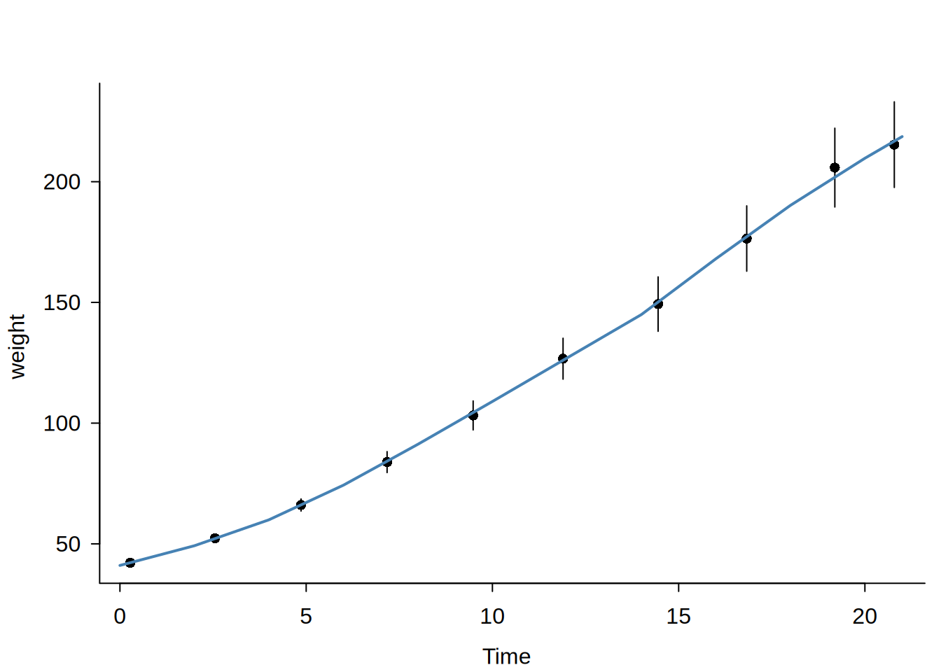
library("dbreg")

#
## In-memory data ----

# Like `dbreg`, we can pass in-memory R data frames to an ephemeral DuckDB
# connection via the `data` argument. 

# Canonical binscatter: bin means (default)
dbbinsreg(weight ~ Time, data = ChickWeight, nbins = 10)

Binscatter Plot
Formula: weight ~ Time 
points = c(0,0) | line = NULL | nbins = 10 (quantile-spaced)
Observations: 578 (original) | 10 (compressed)

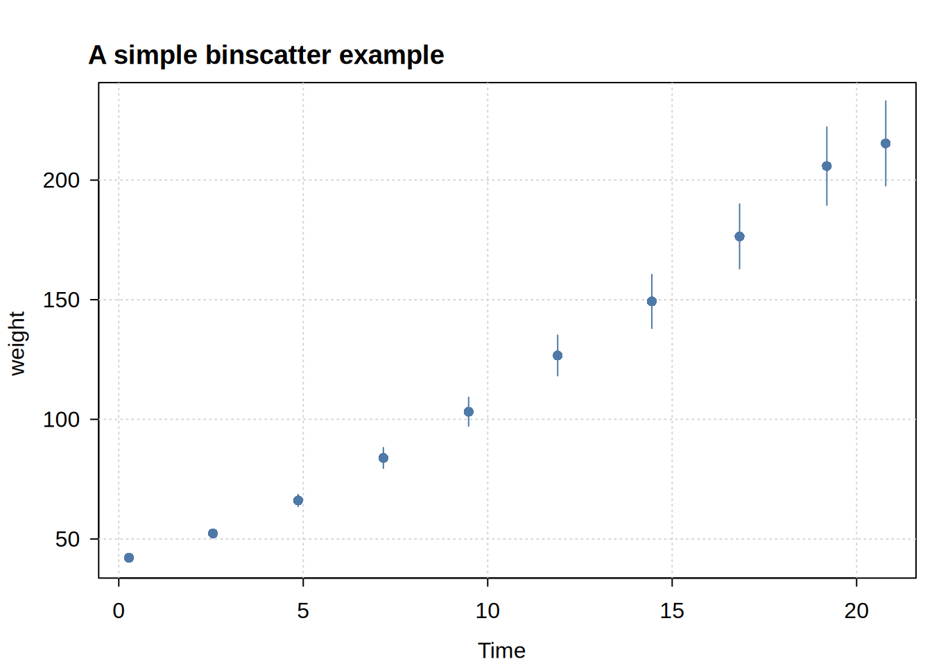
# You can pass additional plotting arguments via ... to (tiny)plot.dbbinsreg
dbbinsreg(weight ~ Time, data = ChickWeight, nbins = 10,
          main = "A simple binscatter example", theme = "clean")

Binscatter Plot
Formula: weight ~ Time 
points = c(0,0) | line = NULL | nbins = 10 (quantile-spaced)
Observations: 578 (original) | 10 (compressed)

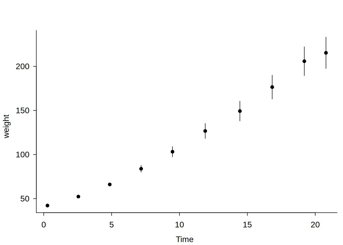
# Alternatively, save the object and plot later
bs = dbbinsreg(weight ~ Time, data = ChickWeight, nbins = 10, plot = FALSE)
plot(bs, main = "Same example, different theme", theme = "classic")

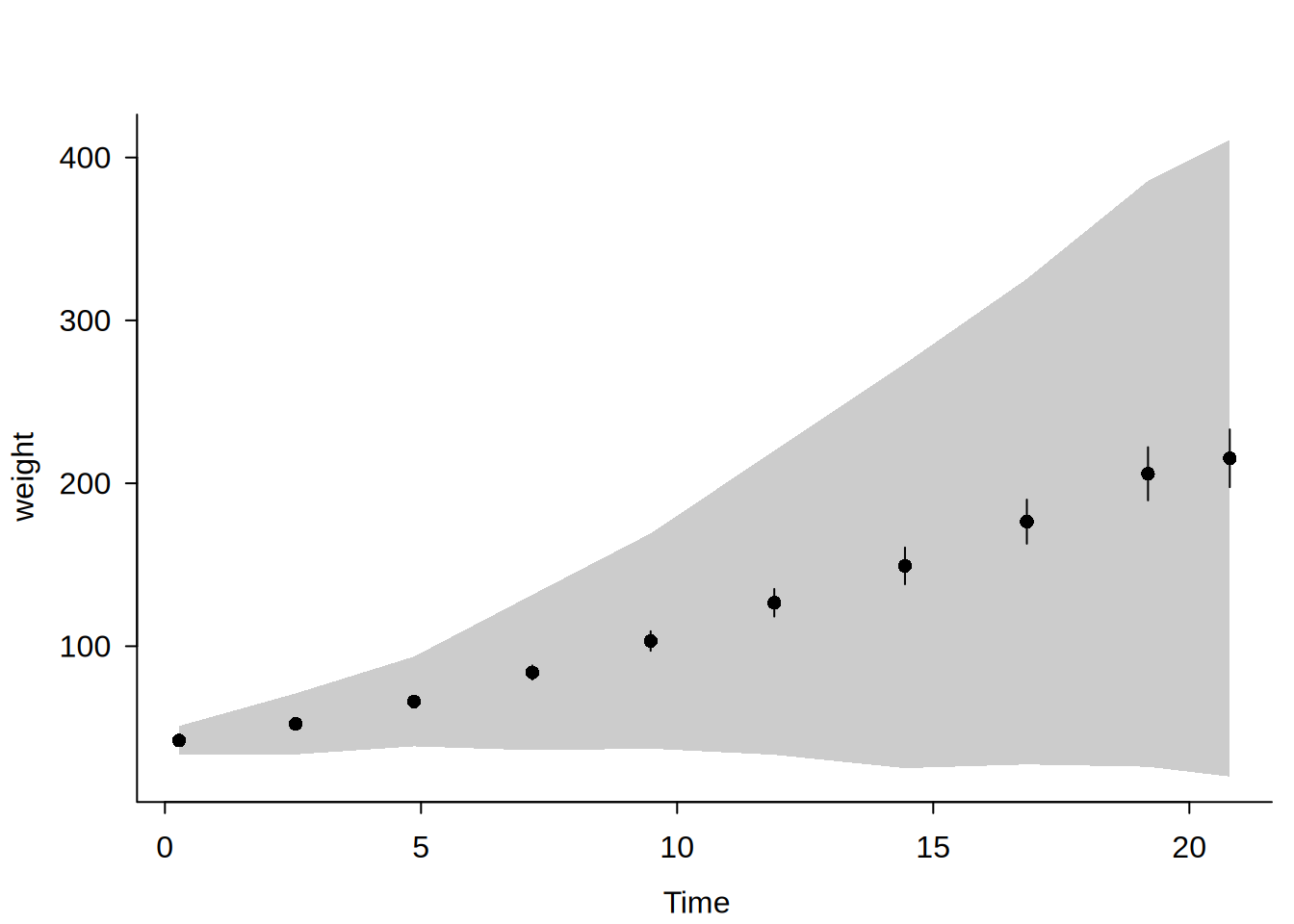
# Piecewise linear (p = 1), no smoothness (s = 0)
dbbinsreg(weight ~ Time, data = ChickWeight, nbins = 10, points = c(1, 0))

Binscatter Plot
Formula: weight ~ Time 
points = c(1,0) | line = NULL | nbins = 10 (quantile-spaced)
Observations: 578 (original) | 21 (compressed)

# Piecewise linear (p = 1) with continuity (s = 1)
dbbinsreg(weight ~ Time, data = ChickWeight, nbins = 10, points = c(1, 1))

Binscatter Plot
Formula: weight ~ Time 
points = c(1,1) | line = NULL | nbins = 10 (quantile-spaced)
N = 578

# With line overlay for smooth visualization
dbbinsreg(weight ~ Time, data = ChickWeight, nbins = 10, points = c(1, 1), line = TRUE)

Binscatter Plot
Formula: weight ~ Time 
points = c(1,1) | line = c(1,1) | nbins = 10 (quantile-spaced)
N = 578

# Different line smoothness to points
dbbinsreg(weight ~ Time, data = ChickWeight, nbins = 10, points = c(0, 0), line = c(1, 1))

Binscatter Plot
Formula: weight ~ Time 
points = c(0,0) | line = c(1,1) | nbins = 10 (quantile-spaced)
Observations: 578 (original) | 10 (compressed)

# With uniform confidence bands (much greater uncertainty)
set.seed(99)
dbbinsreg(weight ~ Time, data = ChickWeight, nbins = 10, cb = TRUE)

Binscatter Plot
Formula: weight ~ Time 
points = c(0,0) | line = NULL | nbins = 10 (quantile-spaced)
Observations: 578 (original) | 10 (compressed)

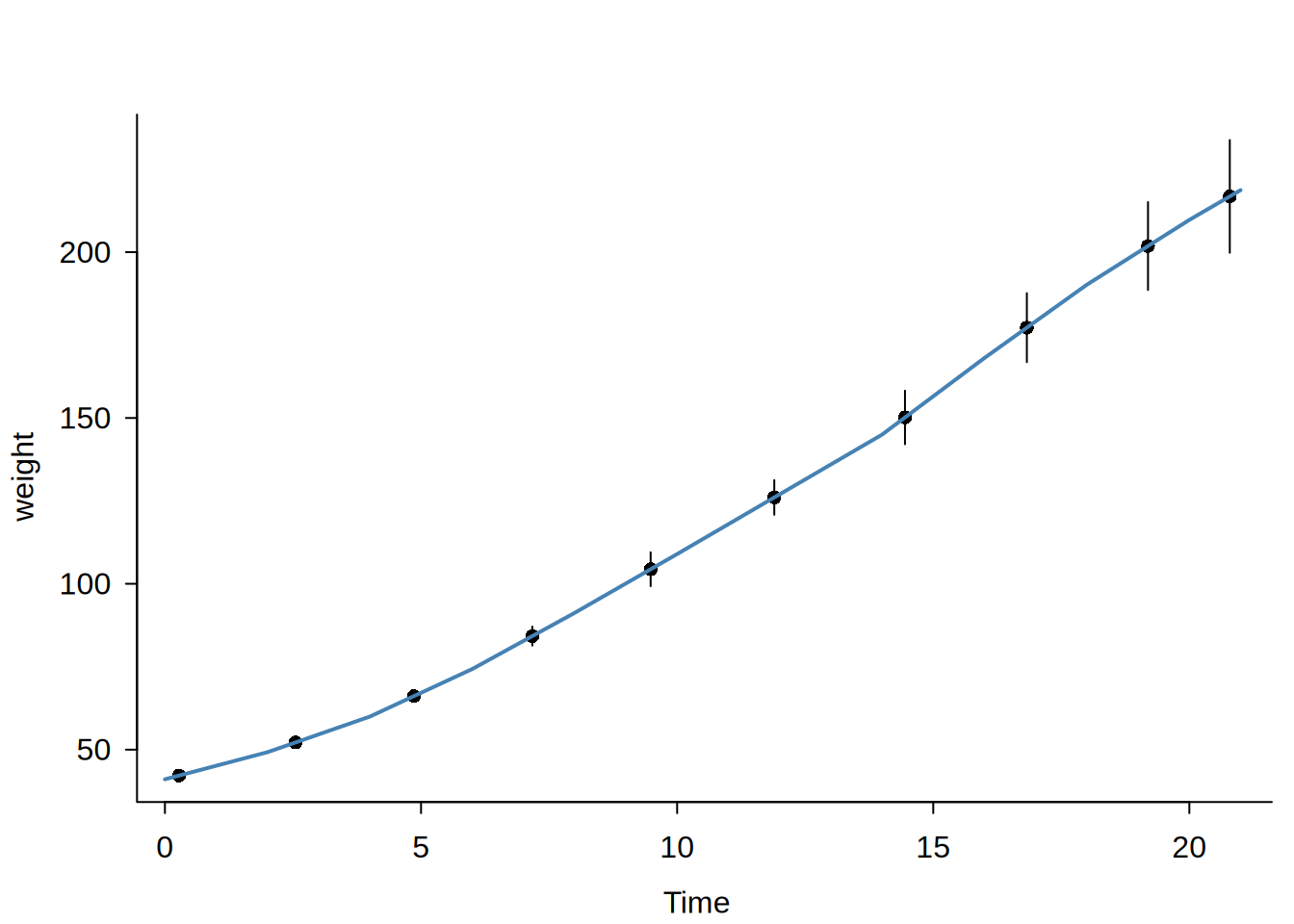
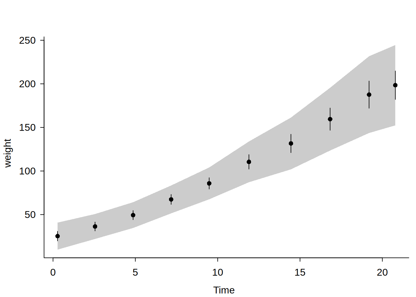
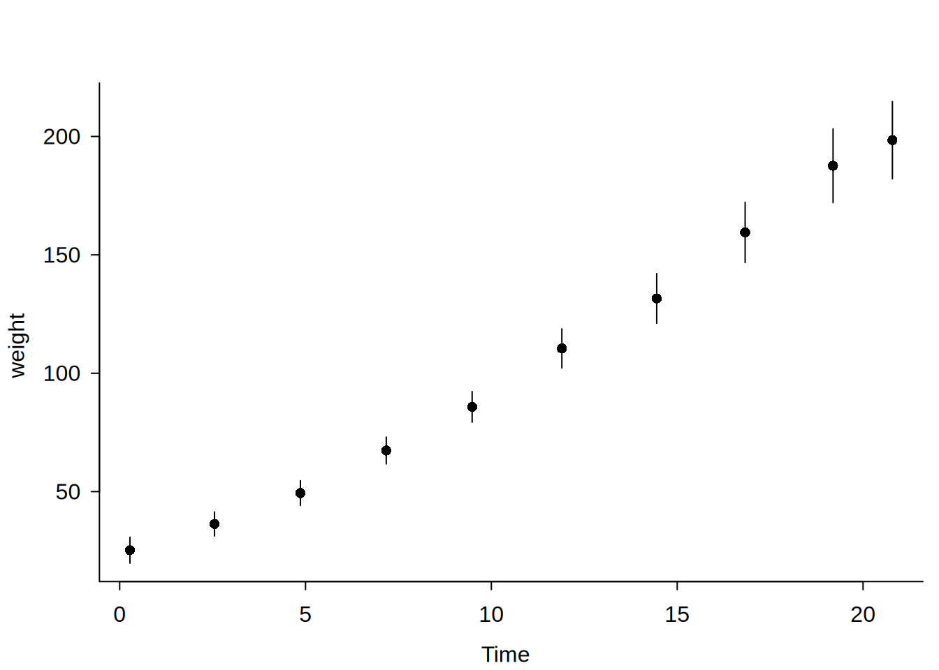
# Accounting for Diet "fixed effects" helps to resolve the situation
# (We'll also add a line and change the theme for a nicer plot)
dbbinsreg(weight ~ Time | Diet, data = ChickWeight, nbins = 10, cb = TRUE,
          line = c(1, 1), theme = "clean")

Binscatter Plot
Formula: weight ~ Time | Diet 
points = c(0,0) | line = c(1,1) | nbins = 10 (quantile-spaced)
Observations: 578 (original) | 40 (compressed)

#
## DBI connection ----

library(DBI)
con = dbConnect(duckdb::duckdb())
dbWriteTable(con, "cw", as.data.frame(ChickWeight))

dbbinsreg(weight ~ Time | Diet, conn = con, table = "cw", nbins = 10,
          theme = "clean")

Binscatter Plot
Formula: weight ~ Time | Diet 
points = c(0,0) | line = NULL | nbins = 10 (quantile-spaced)
Observations: 578 (original) | 40 (compressed)

# etc.

# See ?dbreg for more connection examples

# Clean up
dbDisconnect(con)