dbreg
![]()
![]()
Fast regressions on database backends.
What
dbreg is an R package that leverages the power of databases to run regressions on very large datasets, which may not fit into R’s memory. Various acceleration strategies allow for highly efficient computation, while robust standard errors are computed from sufficient statistics. Our default DuckDB backend provides a powerful, embedded analytics engine to get users up and running with minimal effort. Users can also specify alternative database backends, depending on their computing needs and setup.
The dbreg R package is inspired by, and has similar aims to, the duckreg Python package. This implementation is backend agnostic and also offers some idiomatic, R-focused features like a formula interface and “pretty” print methods. But our long-term goal is that two packages should be aligned in terms of core feature parity.
Install
dbreg can be installed from R-universe.
install.packages(
   "dbreg",
   repos = c("https://grantmcdermott.r-universe.dev", getOption("repos"))
)
We plan to submit dbreg to CRAN in 2026Q1. See our TO-DO list for an idea of what still needs to be completed. Until then, please help us by kicking the tyres and creating GitHub issues for both bug reports and feature requests.
Quickstart
Small dataset
To get ourselves situated, we’ll first demonstrate by using an in-memory R dataset.
library(dbreg)
library(fixest) # for data and comparison

data("trade", package = "fixest")

dbreg(Euros ~ dist_km | Destination + Origin, data = trade, vcov = 'hc1')
#> Compressed OLS estimation, Dep. Var.: Euros
#> Observations.: 38,325 (original) | 210 (compressed)
#> Standard Errors: Heteroskedasticity-robust
#>         Estimate Std. Error t value  Pr(>|t|)
#> dist_km -45709.8    1195.84 -38.224 < 2.2e-16 ***
#> ---
#> Signif. codes:  0 '***' 0.001 '**' 0.01 '*' 0.05 '.' 0.1 ' ' 1
#> RMSE: 124,221,786.3         Adj. R2: 0.215289
Behind the scenes, dbreg has compressed the original dataset down from nearly 40,000 observations to only 210, before running the final (weighted) regression on this much smaller data object. This compression procedure trick follows Wong et al. (2021) and effectively allows us to compute on a much lighter object, saving time and memory. We can confirm that it still gives the same result as running fixest::feols on the full dataset:
feols(Euros ~ dist_km | Destination + Origin, data = trade, vcov = 'hc1')
#> OLS estimation, Dep. Var.: Euros
#> Observations: 38,325
#> Fixed-effects: Destination: 15,  Origin: 15
#> Standard-errors: Heteroskedasticity-robust
#>         Estimate Std. Error t value  Pr(>|t|)
#> dist_km -45709.8    1195.84 -38.224 < 2.2e-16 ***
#> ---
#> Signif. codes:  0 '***' 0.001 '**' 0.01 '*' 0.05 '.' 0.1 ' ' 1
#> RMSE: 124,221,786.3     Adj. R2: 0.215289
#>                       Within R2: 0.025914
Big dataset
For a more appropriate dbreg use-case, let’s run a regression on some NYC taxi data. (Download instructions here.) The dataset that we’re working with here is about 180 million rows deep and takes up 8.5 GB on disk.1 dbreg offers two basic ways to analyse and interact with data of this size.
Option 1: “On-the-fly”
Use the path argument to read the data directly from disk and perform the compression computation in an ephemeral DuckDB connection. This requires that the data are small enough to fit into RAM… but please note that “small enough” is a relative concept. Thanks to DuckDB’s incredible efficiency, your RAM should be able to handle very large datasets that would otherwise crash your R session, and require only a fraction of the computation time. Note that we also invoke the (optional) verbose = TRUE argument to print additional information about the estimation strategy.
dbreg(
   tip_amount ~ fare_amount + passenger_count | month + vendor_name,
   path = "read_parquet('nyc-taxi/**/*.parquet')", ## path to hive-partitioned dataset
   vcov = "hc1",
   verbose = TRUE ## optional (print info about the estimation strategy)
)
#> [dbreg] Auto strategy:
#>         - data has 178,544,324 rows with 2 FE (24 unique groups)
#>         - compression ratio (0.00) satisfies threshold (0.6)
#>         - decision: compress
#> [dbreg] Executing compress strategy SQL
#> Compressed OLS estimation, Dep. Var.: tip_amount
#> Observations.: 178,544,324 (original) | 70,782 (compressed)
#> Standard Errors: Heteroskedasticity-robust
#>                  Estimate Std. Error  t value  Pr(>|t|)
#> fare_amount      0.106744   0.000068 1564.742 < 2.2e-16 ***
#> passenger_count -0.029086   0.000106 -273.866 < 2.2e-16 ***
#> ---
#> Signif. codes:  0 '***' 0.001 '**' 0.01 '*' 0.05 '.' 0.1 ' ' 1
#> RMSE: 1.7                 Adj. R2: 0.243549
Note the size of the original dataset, which is nearly 180 million rows, versus the compressed dataset, which is down to only 70k. On my laptop (M4 MacBook Pro) this regression completes in under 3 seconds… and that includes the time it took to determine an optimal estimation strategy, as well as read the data from disk!2
In case you were wondering, obtaining clustered standard errors is just as easy; simply pass the relevant cluster variable as a formula to the vcov argument. Since we know that the optimal acceleration strategy is "compress", we’ll also go ahead a specify this explicitly to skip the auto strategy overhead.
dbreg(
   tip_amount ~ fare_amount + passenger_count | month + vendor_name,
   path     = "read_parquet('nyc-taxi/**/*.parquet')",
   vcov     = ~month,    # clustered SEs
   strategy = "compress" # skip auto strategy overhead
)
#> Compressed OLS estimation, Dep. Var.: tip_amount
#> Observations.: 178,544,324 (original) | 70,782 (compressed)
#> Standard Errors: Clustered (12 clusters)
#>                  Estimate Std. Error  t value  Pr(>|t|)
#> fare_amount      0.106744   0.000657 162.4934 < 2.2e-16 ***
#> passenger_count -0.029086   0.001030 -28.2278 < 2.2e-16 ***
#> ---
#> Signif. codes:  0 '***' 0.001 '**' 0.01 '*' 0.05 '.' 0.1 ' ' 1
#> RMSE: 1.7                 Adj. R2: 0.243549
Option 2: Persistent database
While querying on-the-fly with our default DuckDB backend is both convenient and extremely performant, you can also run regressions against existing tables in a persistent database connection. This could be DuckDB, but it could also be any other supported backend. All you need to do is specify the appropriate conn and table arguments.
# load the DBI package to connect to a persistent database
library(DBI)

# create connection to persistent DuckDB database (could be any supported backend)
con = dbConnect(duckdb::duckdb(), dbdir = "nyc.db")

# create a 'taxi' table in our new nyc.db database from our parquet dataset
dbExecute(
   con,
   "
   CREATE TABLE taxi AS
      FROM read_parquet('nyc-taxi/**/*.parquet')
      SELECT tip_amount, fare_amount, passenger_count, month, vendor_name
   "
)
#> [1] 178544324

# now run our regression against this conn+table combo
dbreg(
   tip_amount ~ fare_amount + passenger_count | month + vendor_name,
   conn = con,     # database connection,
   table = "taxi", # table name
   vcov = ~month,
   strategy = "compress"
)
#> Compressed OLS estimation, Dep. Var.: tip_amount
#> Observations.: 178,544,324 (original) | 70,782 (compressed)
#> Standard Errors: Clustered (12 clusters)
#>                  Estimate Std. Error  t value  Pr(>|t|)
#> fare_amount      0.106744   0.000657 162.4934 < 2.2e-16 ***
#> passenger_count -0.029086   0.001030 -28.2278 < 2.2e-16 ***
#> ---
#> Signif. codes:  0 '***' 0.001 '**' 0.01 '*' 0.05 '.' 0.1 ' ' 1
#> RMSE: 1.7                 Adj. R2: 0.243549
Result: we get the same coefficient and standard error estimates as earlier.
[!TIP]
Create Temporary Views
If you don’t want to create a persistent database (and materialize data), a nice alternative is
CREATE VIEW. This lets you define subsets or computed columns on-the-fly. For example, to regress on Q1 2012 data with a day-of-week fixed effect:dbExecute(con, " CREATE VIEW nyc_subset AS SELECT tip_amount, trip_distance, passenger_count, vendor_name, month, dayofweek(dropoff_datetime) AS dofw FROM read_parquet('nyc-taxi/**/*.parquet') WHERE year = 2012 AND month <= 3 ") dbreg( tip_amount ~ trip_distance + passenger_count | month + dofw + vendor_name, conn = con, table = "nyc_subset", vcov = ~dofw )
We’ll close by doing some (optional) clean up.
dbRemoveTable(con, "taxi")
dbDisconnect(con)
unlink("nyc.db") # remove from disk
Bonus: Binscatter + interactions
The companion dbbinsreg() function provides a quick way to visualize relationships in large datasets. Here we plot average tips by month:
dbbinsreg(
   tip_amount ~ month, nbins = 12,
   path = "read_parquet('nyc-taxi/**/*.parquet')"
)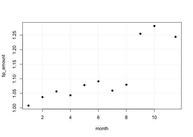
#> Binscatter Plot
#> Formula: tip_amount ~ month
#> points = c(0,0) | line = NULL | nbins = 11 (quantile-spaced)
#> Observations: 178,544,324 (original) | 11 (compressed)
The plot reveals a striking jump in tips starting in September. We can investigate whether this jump differed by taxi vendor using an interaction model. First, create a view with a post-September indicator:
# re-establish a (new) duckdb connection
con = dbConnect(duckdb::duckdb(), shutdown = TRUE)

# create a temporary view with a post-September dummy
dbExecute(
   con,
   "
   CREATE VIEW nyc_post AS
   SELECT
      tip_amount, vendor_name, month,
      CAST(month >= 9 AS INTEGER) AS post
   FROM read_parquet('nyc-taxi/**/*.parquet')
   "
)
#> [1] 0
Then run a DiD-style regression:
dbreg(
   tip_amount ~ post * vendor_name | month,
   conn = con,
   table = "nyc_post"
)
#> Compressed OLS estimation, Dep. Var.: tip_amount
#> Observations.: 178,544,324 (original) | 24 (compressed)
#> Standard Errors: IID
#>                      Estimate Std. Error  t value  Pr(>|t|)
#> post                 0.226457   0.000768 295.0536 < 2.2e-16 ***
#> vendor_nameVTS      -0.009126   0.000349 -26.1327 < 2.2e-16 ***
#> post:vendor_nameVTS  0.006936   0.000615  11.2757 < 2.2e-16 ***
#> ---
#> Signif. codes:  0 '***' 0.001 '**' 0.01 '*' 0.05 '.' 0.1 ' ' 1
#> RMSE: 1.9                 Adj. R2: 0.002497
#> 1 variable was removed because of collinearity (month12)
The results confirm a $0.23 jump in tips post-September, with a small additional increase for VTS taxis.
Acceleration strategies and limitations
All of the examples in this README have made use of the "compress" strategy. But the compression trick is not the only game in town and dbreg supports several other acceleration strategies: "moments", "demean", and "mundlak". Depending on your data and regression requirements, one of these other strategies may better suit your problem. The good news is that (the default) strategy = "auto" option uses some intelligent heuristics to determine which strategy is (probably) optimal for each case. You can set the verbose = TRUE argument to get real-time feedback about the decision criteria being used. The Acceleration Strategies section of the ?dbreg helpfile contains a lot of detail about the different options and tradeoffs involved, so please do consult the documentation.
In brief, we can say that dbreg works best when the fixed effects are low-dimensional relative to the data size, yielding high compression ratios, which in turn enable the remarkable speed-ups that we have demonstrated above. In the specific case of the NYC taxi data, we are able to compress 180 million rows down to just 70k observations exactly because the FE groups (month × vendor) only have 24 unique combinations. Compression becomes less effective for “true” panel data (repeated cross sections) with high-dimensional unit and time FE, where N >> T. In such cases, grouping by (X, unit, time) yields little to no compression since each combination is essentially unique. The "demean" and "mundlak" strategies provide a nice alternative here, since they reduce dimensionality by taking covariate averages. While this is not as efficient as the "compress" approach, all computation is done on the database backend and this means we can run really big regressions without crashing our R session.
Please note that fixest remains an excellent choice for datasets that fit in R’s memory, especially for high-dimensional FE problems where its iterative demeaning algorithm remains best in class.
Acknowledgements
dbreg is indebted to the following open-source projects:
- duckreg (Lal et al., 2024). The original Python package that inspired this R implementation.
- etwfe (McDermott). A prior R implementation that employs compression-based estimation (albeit in a narrower context).
- fixest (Bergé et al, 2026). For its elegant formula syntax and user API, which we deliberately try to emulate alongside its performance philosophy.
- DBI (R-SIG-DB, Wickham & Müller). The R database interface layer, which handles all of our SQL parsing and backend connectivity under the hood.
- DuckDB (Mühleisen & Raasveldt). The amazingly powerful embedded analytics engine, which powers all of our default operations.
We also build on the following theory papers:
Footnotes
To be clear, this dataset would occupy significantly more RAM than 8.5 GB if we loaded it into R’s memory, due to data serialization and the switch to richer representation formats (e.g., ordered factors require more memory). So there’s a good chance that just trying to load this raw dataset into R would cause your whole system to crash… never mind doing any statistical analysis on it.↩︎
If we provided an explicit
dbreg(..., strategy = "compress")argument (thus skipping the automatic strategy determination), then the total computation time drops to less than 1 second…↩︎