Run a binscatter regression on a database backend and plot the result

Description

Performs binned regression entirely in SQL, returning plot-ready data with estimated bin means or piecewise polynomial fits. The API is designed to be compatible with the binsreg package by Cattaneo, Crump, Farrell, and Feng (2024). Supports unconditional and conditional models (with controls and/or fixed effects).

Usage

dbbinsreg(
  fml,
  conn = NULL,
  table = NULL,
  data = NULL,
  path = NULL,
  points = c(0, 0),
  line = NULL,
  linegrid = 20,
  nbins = 20,
  binspos = "qs",
  randcut = NULL,
  sample_fit = NULL,
  ci = TRUE,
  cb = FALSE,
  vcov = NULL,
  level = 0.95,
  nsims = 500,
  strategy = c("auto", "compress"),
  plot = TRUE,
  verbose = getOption("dbreg.verbose", FALSE),
  dots = NULL
)

Arguments

fml

A formula representing the binscatter relation. The first variable on the RHS is the running variable; additional variables are controls. Fixed effects go after |. Examples:

  • y ~ x: simple binscatter

  • y ~ x + w1 + w2: binscatter with controls

  • y ~ x | fe: binscatter with fixed effects

  • y ~ x + w1 + w2 | fe: binscatter with controls and fixed effects

conn Database connection, e.g. created with dbConnect. Can be either persistent (disk-backed) or ephemeral (in-memory). If no connection is provided, then an ephemeral duckdb connection will be created automatically and closed before the function exits. Note that a persistent (disk-backed) database connection is required for larger-than-RAM datasets in order to take advantage of out-of-core functionality like streaming (where supported).
table, data, path

Mutually exclusive arguments for specifying the data table (object) to be queried. In order of precedence:

  • table: Character string giving the name of the data table in an existing (open) database connection.

  • data: R dataframe that can be copied over to conn as a temporary table for querying via the DuckDB query engine. Ignored if table is provided.

  • path: Character string giving a path to the data file(s) on disk, which will be read into conn. Internally, this string is passed to the FROM query statement, so could (should) include file globbing for Hive-partitioned datasets, e.g. “mydata/**/.*parquet”. For more precision, however, it is recommended to pass the desired database reader function as part of this string, e.g. “read_parquet(’mydata/**/*.parquet’)“ for DuckDB; note the use of single quotes. Ignored if either table or data is provided.

points A vector c(p, s) specifying the polynomial degree \(p\) and smoothness \(s\) for the points (point estimates at bin means). Default is c(0, 0) for canonical binscatter (bin means). Set to NULL or FALSE to suppress points. The smoothness s must satisfy s <= p.
line A vector c(p, s) specifying the polynomial degree \(p\) and smoothness \(s\) for the line (evaluated on a grid within bins). Default is NULL (no line). Set to TRUE for c(0, 0) or a vector like c(1, 1) for piecewise linear with continuity constraints. The smoothness \(s\) must satisfy s <= p.
linegrid Number of evaluation points per bin for the line. Default is 20.
nbins Integer number of bins. Default is 20.
binspos Bin positioning method. One of either “qs” (quantile-spaced, equal-count bins, the default), “es” (evenly-spaced, equal-width bins), or a numeric vector of knot positions for manual specification.
randcut Numeric in the range (0,1]. Controls the random sampling fraction for bin boundary computation on large datasets. If NULL (the default), then sampling is automatic: 0.01 (1%) for datasets exceeding 1 million rows and 1 (100%) otherwise. Note that sampling is only used for computing the bin boundaries, since this requires an expensive ranking operation. The subsequent, primary regression operations use all of the data (unless sample_fit is enabled).
sample_fit Logical or NULL. Controls whether the spline regression (s > 0) re-uses the same random sample (controlled by randcut) that is used for computing the bin boundaries. This trades off some precision for major speed gains on big datasets; see the Smoothness Constraints section below. If NULL (the default), sampling is enabled automatically when applicable, with a message. Explicitly set to TRUE to enable the same sampling behaviour, but without the message. Alternatively, set to FALSE to use the full dataset. Ignored when s = 0, since the “compress” strategy already handles these aggregation cases efficiently.
ci Logical. Calculate standard errors and confidence intervals for points? Default is TRUE.
cb Logical. Calculate simultaneous confidence bands using simulation? Default is FALSE.
vcov Character string or formula for standard errors. Options are “HC1” (default, heteroskedasticity-robust, matches binsreg), “iid”, or a one-sided formula for clustered standard errors (e.g., ~cluster_var).
level Numeric in the range [0,1], giving the confidence level for the confidence levels and/or bands. Default is 0.95.
nsims Number of simulation draws for confidence band computation. Default is 500. Only used when cb = TRUE.
strategy Acceleration strategy passed to dbreg. Only “compress” is currently supported; “auto” (the default) maps to “compress”. Included for API consistency with dbreg. Ignored when smoothness s > 0, since spline basis construction requires row-level data (i.e., no pre-aggregation).
plot Logical. If TRUE (default), a plot is produced as a side effect. Set to FALSE to suppress plotting.
verbose Logical. Print auto strategy and progress messages to the console? Defaults to FALSE. This can be overridden for a single call by supplying verbose = TRUE, or set globally via options(dbreg.verbose = TRUE).
dots Alias for points for binsreg compatibility. If not NULL, overrides the points argument.

Value

A list of class "dbbinsreg" containing:

points
Data frame of the point estimates (one row per bin): x (bin mean), bin, and fit (fitted value). If ci=TRUE in the original call, then also includes the columns: se, lwr, and upr. Similarly, if cb=TRUE, then includes the columns: cb_lwr and cb_upr.
line
Data frame of the line estimates (multiple rows per bin): x, bin, fit. Only present if line is specified.
bins
Data frame with bin boundaries: id (bin number), left (left endpoint), right (right endpoint).
model
The fitted dbreg model object (for points).
opt
List of options used: points, line, nbins, binspos, etc.

If plot = TRUE (the default), a binscatter plot is also produced as a side effect. See plot.dbbinsreg for plot customization.

Comparison with binsreg

The dbbinsreg function is deeply inspired by the binsreg package (Cattaneo et. al., 2024). The main difference is that dbbinsreg performs most of its computation on a database backend, employing various acceration strategies, which makes it particularly suitable for large datasets (which may not fit in memory). At the same time, the database backend introduces its own set of tradeoffs. We cover the most important points of similarity and difference below.

Core API and bin selection

We aim to mimic the binsreg API as much as possible. Key parameter mappings include:

  • points (alias dots): Point estimates at bin means

    • c(0,0): Canonical binscatter (bin means)

    • c(p,0): Piecewise polynomial of degree \(p\), no smoothness

    • c(p,s): Piecewise polynomial with \(s\) smoothness constraints

  • line: Same as points but evaluated on a finer grid for smooth visualization

  • binspos: Bin positioning

    • “qs”: Quantile-spaced (equal count)

    • “es”: Evenly-spaced (equal width)

Important: Unlike binsreg, dbbinsreg does not automatically select the IMSE-optimal number of bins. Rather, users must specify nbins manually (with a default of value of 20). For guidance on bin selection, see binsregselect or Cattaneo et al. (2024).

Smoothness constraints

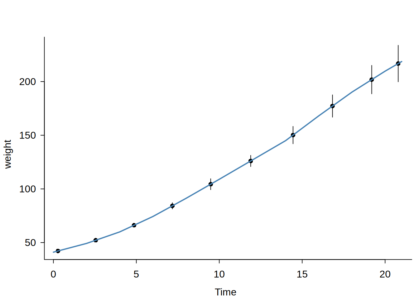
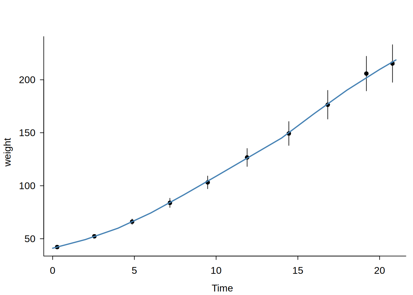
When s > 0, the function fits a regression spline using a truncated power basis. For degree \(p\) and smoothness \(s\), the basis includes global polynomial terms (\(x, x^2, \ldots, x^p\)) plus truncated power terms \((x - \kappa_j)_+^r\) at each interior knot \(\kappa_j\) for \(r = s, \ldots, p\). This enforces \(C^{s-1}\) continuity (continuous derivatives up to order \(s-1\)) at bin boundaries. For example, c(1,1) gives a piecewise linear fit that is continuous; c(2,2) gives a piecewise quadratic with continuous first derivatives.

Important: Unlike s = 0 (which uses the “compress” strategy for fast aggregation), s > 0 requires row-level spline basis construction and can be very slow on large datasets. As a result, dbbinsreg re-uses the random sample (used to compute the bin boundaries) for estimating the spline fits in these cases, ensuring much faster computation at the cost of reduced precision. Users can override this behaviour by passing the sample_fit = FALSE argument to rather estimate the spline regressions on the full dataset.

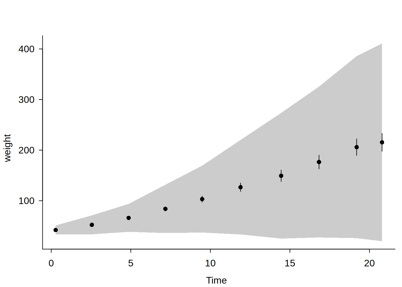
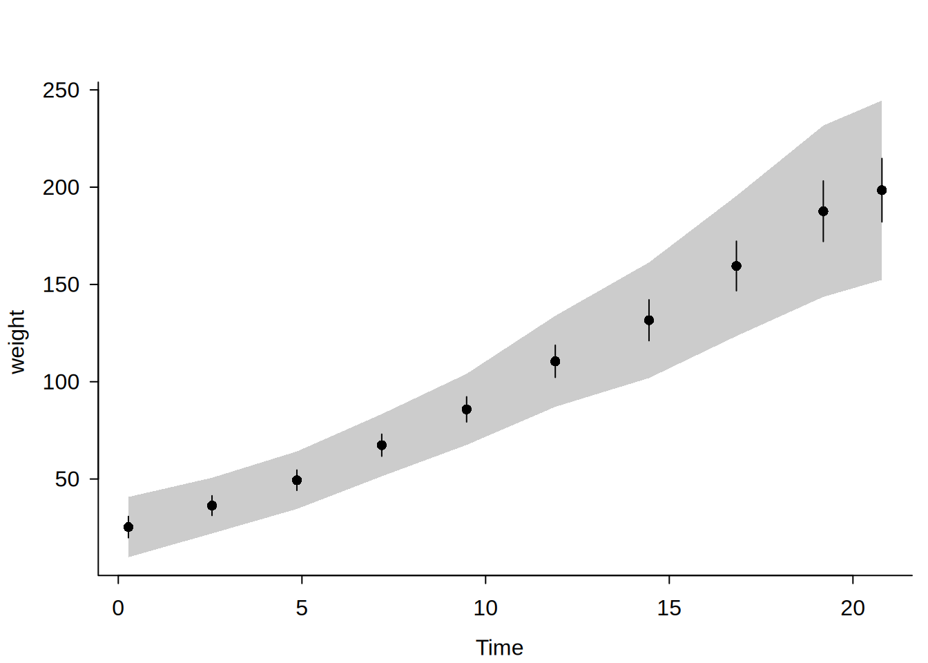
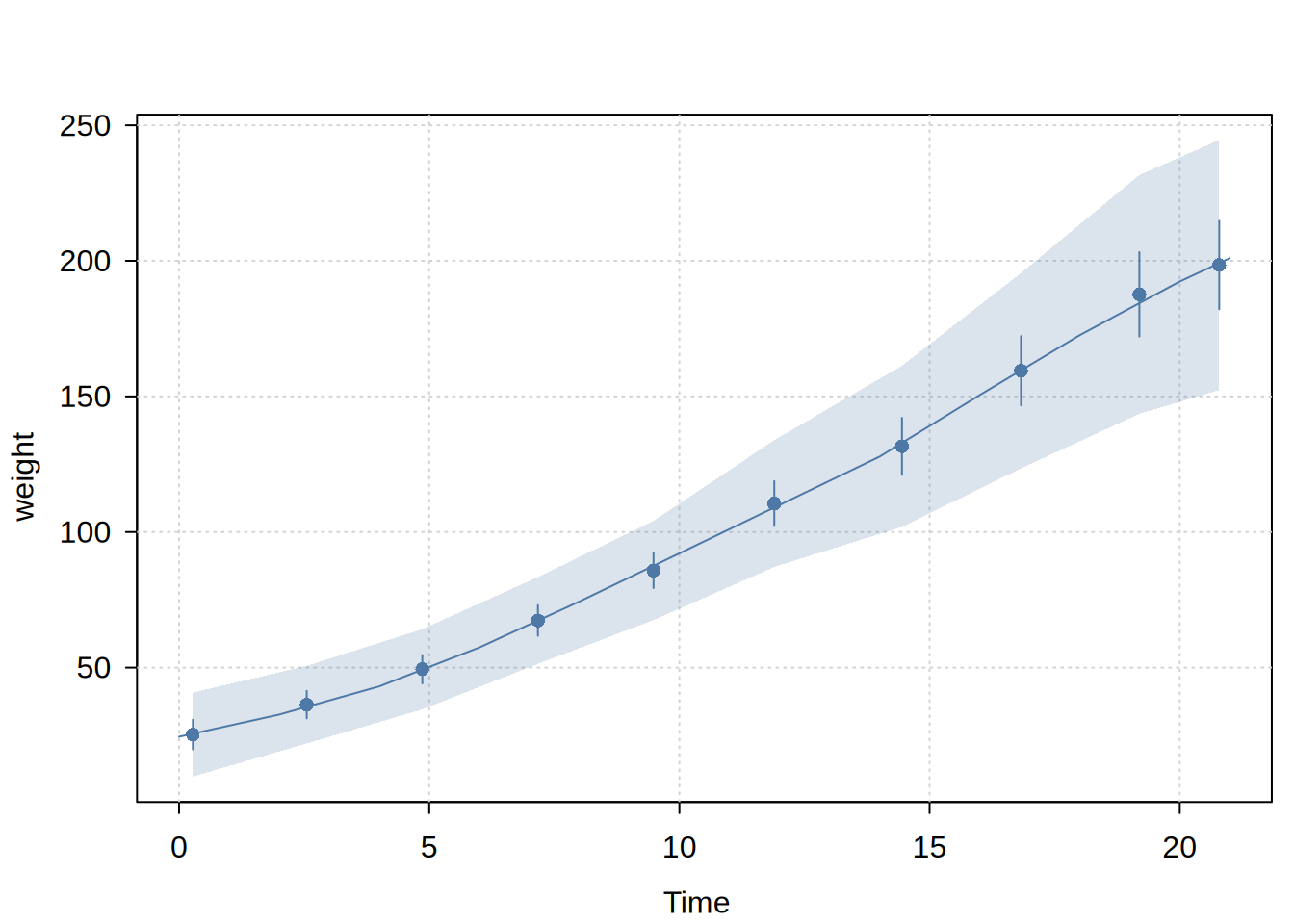
Confidence intervals vs confidence bands

When ci = TRUE (default), pointwise confidence intervals (CIs) are computed at each bin mean using standard asymptotic theory. When cb = TRUE, simultaneous confidence bands (CBs) are computed using a simulation-based sup-\(t\) procedure:

  1. Draw nsims samples from the asymptotic distribution of the estimator

  2. Compute the supremum of the \(t\)-statistics across all bins for each draw

  3. Use the (\(1-\alpha\)) quantile of these suprema as the critical value

The confidence band is wider than pointwise CIs and provides simultaneous coverage: with (\(1-\alpha\)) probability, the entire true function lies within the band. This is useful for making statements about the overall shape of the relationship rather than individual point estimates.

There are two important caveats, regarding dbbinsreg’s CB support:

  • Unlike binsreg, which evaluates CB on a fine grid within each bin, dbbinsreg computes CB only at bin means (same points as CI). This is much simpler for our backend SQL implementation and should be sufficient for most applications.

  • CBs are currently only supported for unconstrained estimation (smoothness s = 0). When cb = TRUE with s > 0, a warning is issued and CB is skipped.

Note on quantile bin boundaries

When using quantile-spaced bins (binspos = “qs”), dbbinsreg uses SQL’s NTILE() window function, while binsreg uses R’s quantile with type = 2. These algorithms have slightly different tie-breaking behavior, which can cause small differences in bin assignments at boundaries. In practice, differences are typically <1% and become negligible with larger datasets. To match binsreg exactly, compute quantile breaks on a subset of data in R and pass them via the binspos argument as a numeric vector.

References

Cattaneo, M. D., R. K. Crump, M. H. Farrell, and Y. Feng (2024). On Binscatter. American Economic Review, 114(5): 1488-1514.

See Also

plot.dbbinsreg for plot customization, dbreg for the underlying regression engine, binsreg for the original implementation.

Examples

library("dbreg")

#
## In-memory data ----

# Like `dbreg`, we can pass in-memory R data frames to an ephemeral DuckDB
# connection via the `data` argument. 

# Canonical binscatter: bin means (default)
dbbinsreg(weight ~ Time, data = ChickWeight, nbins = 10)

Binscatter Plot
Formula: weight ~ Time 
points = c(0,0) | line = NULL | nbins = 10 (quantile-spaced)
Observations: 578 (original) | 10 (compressed)
# For plot customization, save the model object so you can pass additional args
# to (tiny)plot.dbbinsreg
bs = dbbinsreg(weight ~ Time, data = ChickWeight, nbins = 10)
plot(bs, theme = "clean", main = "A simple binscatter example")

# Alternatively: you can also set a global (tiny)plot theme
tinyplot::tinytheme("classic")

# Piecewise linear (p = 1), no smoothness (s = 0)
dbbinsreg(weight ~ Time, data = ChickWeight, nbins = 10, points = c(1, 0))

Binscatter Plot
Formula: weight ~ Time 
points = c(1,0) | line = NULL | nbins = 10 (quantile-spaced)
Observations: 578 (original) | 21 (compressed)
# Piecewise linear (p = 1) with continuity (s = 1)
dbbinsreg(weight ~ Time, data = ChickWeight, nbins = 10, points = c(1, 1))
Binscatter Plot
Formula: weight ~ Time 
points = c(1,1) | line = NULL | nbins = 10 (quantile-spaced)
N = 578
# With line overlay for smooth visualization
dbbinsreg(weight ~ Time, data = ChickWeight, nbins = 10, points = c(1, 1), line = TRUE)

Binscatter Plot
Formula: weight ~ Time 
points = c(1,1) | line = c(1,1) | nbins = 10 (quantile-spaced)
N = 578
# Different line smoothness to points
dbbinsreg(weight ~ Time, data = ChickWeight, nbins = 10, points = c(0, 0), line = c(1, 1))

Binscatter Plot
Formula: weight ~ Time 
points = c(0,0) | line = c(1,1) | nbins = 10 (quantile-spaced)
Observations: 578 (original) | 10 (compressed)
# With uniform confidence bands (much greater uncertainty)
set.seed(99)
dbbinsreg(weight ~ Time, data = ChickWeight, nbins = 10, cb = TRUE)

Binscatter Plot
Formula: weight ~ Time 
points = c(0,0) | line = NULL | nbins = 10 (quantile-spaced)
Observations: 578 (original) | 10 (compressed)
# Accounting for Diet "fixed effects" helps to resolve the situation
dbbinsreg(weight ~ Time | Diet, data = ChickWeight, nbins = 10, cb = TRUE)

Binscatter Plot
Formula: weight ~ Time | Diet 
points = c(0,0) | line = NULL | nbins = 10 (quantile-spaced)
Observations: 578 (original) | 40 (compressed)
#
## DBI connection ----

library(DBI)
con = dbConnect(duckdb::duckdb())
dbWriteTable(con, "cw", as.data.frame(ChickWeight))

dbbinsreg(weight ~ Time | Diet, conn = con, table = "cw", nbins = 10)

Binscatter Plot
Formula: weight ~ Time | Diet 
points = c(0,0) | line = NULL | nbins = 10 (quantile-spaced)
Observations: 578 (original) | 40 (compressed)
# etc.

# See ?dbreg for more connection examples

# Clean up
dbDisconnect(con)
tinyplot::tinytheme() # reset plot theme