
Marginal effects and interaction terms
The trick
I recently tweeted one of my favourite R tricks for getting the full marginal effect(s) of interaction terms. The short version is that, instead of writing your model as lm(y ~ f1 * x2), you write it as lm(y ~ f1 / x2). Here’s an example using everyone’s favourite mtcars dataset.
First, partial marginal effects with the standard f1 * x2 interaction syntax.
summary(lm(mpg ~ factor(am) * wt, mtcars))##
## Call:
## lm(formula = mpg ~ factor(am) * wt, data = mtcars)
##
## Residuals:
## Min 1Q Median 3Q Max
## -3.600 -1.545 -0.533 0.901 6.091
##
## Coefficients:
## Estimate Std. Error t value Pr(>|t|)
## (Intercept) 31.416 3.020 10.40 4.0e-11 ***
## factor(am)1 14.878 4.264 3.49 0.0016 **
## wt -3.786 0.786 -4.82 4.6e-05 ***
## factor(am)1:wt -5.298 1.445 -3.67 0.0010 **
## ---
## Signif. codes: 0 '***' 0.001 '**' 0.01 '*' 0.05 '.' 0.1 ' ' 1
##
## Residual standard error: 2.59 on 28 degrees of freedom
## Multiple R-squared: 0.833, Adjusted R-squared: 0.815
## F-statistic: 46.6 on 3 and 28 DF, p-value: 5.21e-11Second, full marginal effects with the trick f1 / x2 interaction syntax.
summary(lm(mpg ~ factor(am) / wt, mtcars))##
## Call:
## lm(formula = mpg ~ factor(am)/wt, data = mtcars)
##
## Residuals:
## Min 1Q Median 3Q Max
## -3.600 -1.545 -0.533 0.901 6.091
##
## Coefficients:
## Estimate Std. Error t value Pr(>|t|)
## (Intercept) 31.416 3.020 10.40 4.0e-11 ***
## factor(am)1 14.878 4.264 3.49 0.0016 **
## factor(am)0:wt -3.786 0.786 -4.82 4.6e-05 ***
## factor(am)1:wt -9.084 1.212 -7.49 3.7e-08 ***
## ---
## Signif. codes: 0 '***' 0.001 '**' 0.01 '*' 0.05 '.' 0.1 ' ' 1
##
## Residual standard error: 2.59 on 28 degrees of freedom
## Multiple R-squared: 0.833, Adjusted R-squared: 0.815
## F-statistic: 46.6 on 3 and 28 DF, p-value: 5.21e-11To get the full marginal effect of factor(am)1:wt in the first case, I have to manually sum up the coefficients on the constituent parts (i.e. factor(am)1=14.8784 + factor(am)1:wt=-5.2984). In the second case, I get the full marginal effect of −9.0843 immediately in the model summary. Not only that, but the correct standard errors, p-values, etc. are also automatically calculated for me. (If you don’t remember, manually calculating SEs for multiplicative interaction terms is a huge pain. And that’s before we even get to complications like standard error clustering.)
Note that the lm(y ~ f1 / x2) syntax is actually shorthand for the more verbose lm(y ~ f1 + f1:x2). I’ll get back to this point further below, but I wanted to flag the expanded syntax as important because it demonstrates why this trick “works”. The key idea is to drop the continuous variable parent term (here: x2) from the regression. This forces all of the remaining child terms relative to the same base. It’s also why this trick can easily be adapted to, say, Julia or Stata (see here).
So far, so good. It’s a great trick that has saved me a bunch of time (say nothing of likely user-error) that I recommend to everyone. Yet, I was prompted to write a separate blog post after being asked whether this trick a) works for higher-order interactions, and b) other non-linear models like logit? The answer in both cases is a happy “Yes!”.
Dealing with higher-order interactions
Let’s consider a threeway interaction, since this will demonstrate the general principle for higher-order interactions. First, as a matter of convenience, I’ll create a new dataset so that I don’t have to keep specifying the factor variables.
mtcars2 = mtcars
mtcars2$vs = factor(mtcars2$vs); mtcars2$am = factor(mtcars2$am)
Now, we run a threeway interaction and view the (naive, partial) marginal effects.
fit1 = lm(mpg ~ am * vs * wt, mtcars2)
summary(fit1)
##
## Call:
## lm(formula = mpg ~ am * vs * wt, data = mtcars2)
##
## Residuals:
## Min 1Q Median 3Q Max
## -3.305 -1.715 -0.728 1.350 5.362
##
## Coefficients:
## Estimate Std. Error t value Pr(>|t|)
## (Intercept) 25.059 4.040 6.20 2.1e-06 ***
## am1 17.304 7.704 2.25 0.034 *
## vs1 6.468 10.144 0.64 0.530
## wt -2.439 0.969 -2.52 0.019 *
## am1:vs1 -4.705 12.976 -0.36 0.720
## am1:wt -5.475 2.467 -2.22 0.036 *
## vs1:wt -0.937 3.056 -0.31 0.762
## am1:vs1:wt 1.083 4.442 0.24 0.809
## ---
## Signif. codes: 0 '***' 0.001 '**' 0.01 '*' 0.05 '.' 0.1 ' ' 1
##
## Residual standard error: 2.47 on 24 degrees of freedom
## Multiple R-squared: 0.87, Adjusted R-squared: 0.832
## F-statistic: 23 on 7 and 24 DF, p-value: 3.53e-09Say we are interested in the full marginal effect of the threeway interaction vs1:am1:wt. Even summing the correct parent coefficients is a potentially error-prone process of thinking through the underlying math (which terms are excluded from the partial derivative, etc.) And don’t even get me started on the standard errors…
Now, it should be said that there are several existing tools for obtaining this number that don’t require us working through everything by hand. Here I’ll use my favourite such tool — the margins package — to save me the mental arithmetic.
library(margins)
library(magrittr) ## for the pipe operator

fit1 %>%
  margins(
    variables = "wt",
    at = list(vs = "1", am = "1")
    ) %>%
  summary()
## factor vs am AME SE z p lower upper
## wt 1.0000 1.0000 -7.7676 2.2903 -3.3916 0.0007 -12.2565 -3.2788We now at least see that the full (average) marginal effect is −7.7676. Still, while this approach works well in the present example, we can also begin to see some downsides. It requires extra coding steps and comes with its own specialised syntax. Moreover, underneath the hood, margins relies on a numerical delta method that can dramatically increase computation time and memory use for even moderately sized real-world problems. (Is your dataset bigger than 1 GB? Good luck.) Another practical problem is that margins may not even support your model class. (See here.)
So, what about the alternative? Does our little syntax trick work here too? The good news is that, yes, it’s just as simple as it was before.
fit2 = lm(mpg ~ am / vs / wt, mtcars2)
summary(fit2)
##
## Call:
## lm(formula = mpg ~ am/vs/wt, data = mtcars2)
##
## Residuals:
## Min 1Q Median 3Q Max
## -3.305 -1.715 -0.728 1.350 5.362
##
## Coefficients:
## Estimate Std. Error t value Pr(>|t|)
## (Intercept) 25.059 4.040 6.20 2.1e-06 ***
## am1 17.304 7.704 2.25 0.0342 *
## am0:vs1 6.468 10.144 0.64 0.5298
## am1:vs1 1.763 8.092 0.22 0.8294
## am0:vs0:wt -2.439 0.969 -2.52 0.0189 *
## am1:vs0:wt -7.914 2.268 -3.49 0.0019 **
## am0:vs1:wt -3.376 2.898 -1.16 0.2555
## am1:vs1:wt -7.768 2.290 -3.39 0.0024 **
## ---
## Signif. codes: 0 '***' 0.001 '**' 0.01 '*' 0.05 '.' 0.1 ' ' 1
##
## Residual standard error: 2.47 on 24 degrees of freedom
## Multiple R-squared: 0.87, Adjusted R-squared: 0.832
## F-statistic: 23 on 7 and 24 DF, p-value: 3.53e-09Again, we get the full marginal effect of −7.7676 (and correct SE of 2.2903) directly in the model object. Much easier, isn’t it?
Where this approach really shines is in combination with plotting. Say, after extracting the coefficients with broom::tidy(), or simply plotting them directly with modelsummary::modelplot(). Model results are usually much easier to interpret visually, but this is precisely where we want to depict full marginal effects to our reader. Here I’ll use the modelsummary package to produce a nice coefficient plot of our threeway interaction terms.
library(modelsummary)
library(ggplot2)    ## for some extra ggplot2 layers
library(hrbrthemes) ## theme(s) I like

## Optional: A dictionary of "nice" coefficient names for our plot
dict = c('am0:vs0:wt' = 'Manual\nStraight',
         'am0:vs1:wt' = 'Manual\nV-shaped',
         'am1:vs0:wt' = 'Automatic\nStraight',
         'am1:vs1:wt' = 'Automatic\nV-shaped')

modelplot(fit2, coef_map = dict) +
  geom_vline(xintercept = 0, col = "orange") +
  labs(
    x = "Marginal effect (Δ in MPG : Δ in '000 lbs)",
    title = " Marginal effect of vehicle weight on MPG",
    subtitle = "Conditional on transmission type and engine shape"
    ) +
theme_ipsum() 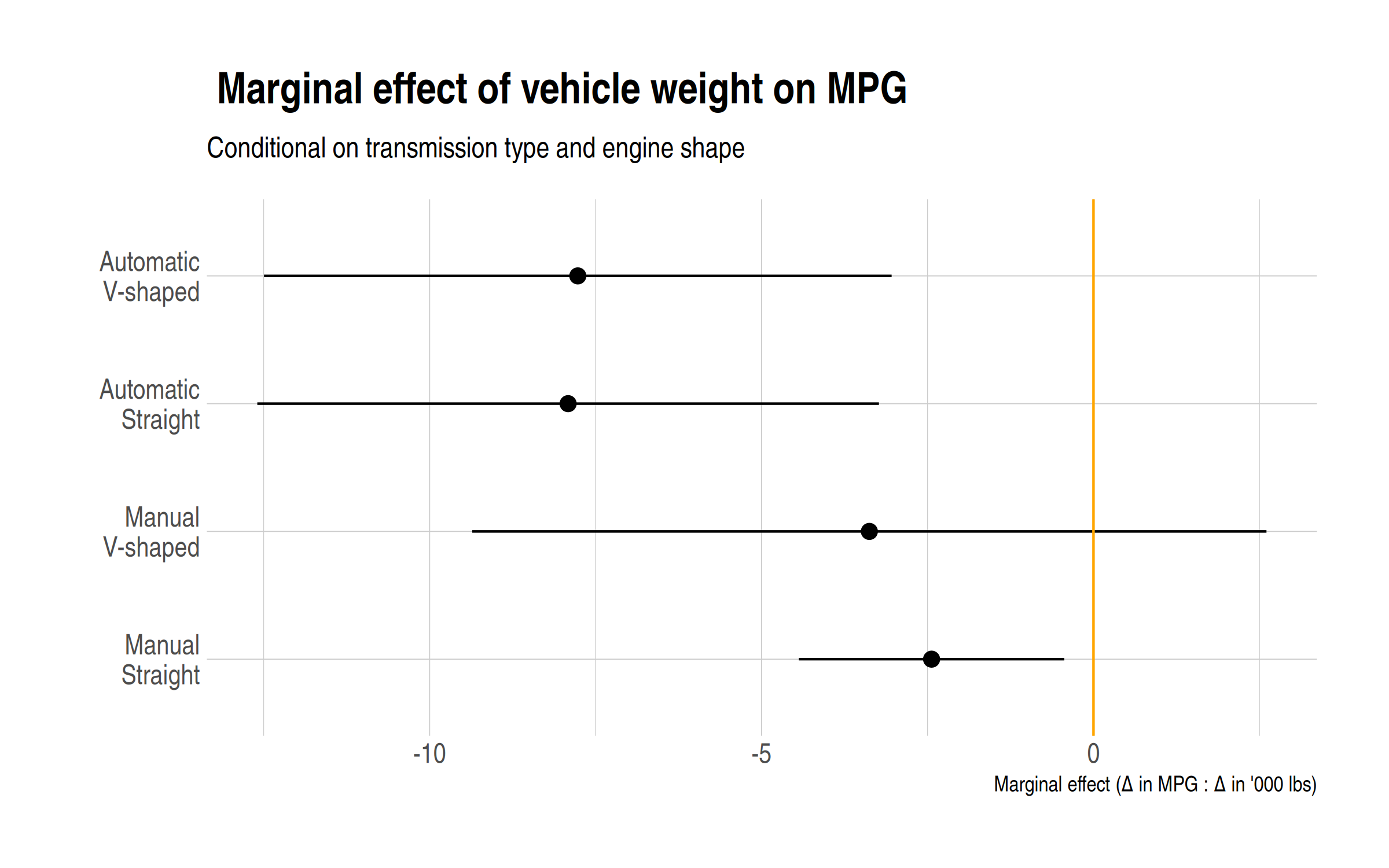
The above plot immediately makes clear how automatic transmission exacerbates the impact of vehicle weight on MPG. We also see that the conditional impact of engine shape is more ambiguous. In contrast, I invite you to produce an equivalent plot using our earlier fit1 object and see if you can easily make sense of it. (I certainly can’t.)
Aside: Specifying (parent) terms as fixed effects
On the subject of speed, recall that the lm(y ~ f1 / x2) syntax is equivalent to the more verbose lm(y ~ f1 + f1:x2). This verbose syntax provides a clue for greatly reducing computation time for large models; particularly those with factor variables that contain many levels. We simply need specify the parent factor terms as fixed effects (using a specialised library like fixest). Going back to our introductory twoway interaction example, you would thus write the model as follows.
library(fixest)
feols(mpg ~ am:wt | am, mtcars2)
(I’ll let you confirm for yourself that running the above models gives the correct −9.0843 figure from before.)
In case you’re wondering, the verbose equivalent for the f1 / f2 / x3 threeway interaction is f1 + f2 + f1:f2 + f1:f2:x3. So we can use the same FE approach for this more complicated case as follows.1
## Option 1 using verbose base lm(). Not run.
# summary(lm(mpg ~ am + vs + am:vs + am:vs:wt, mtcars2))

## Option 2 using fixest::feols()
feols(mpg ~ am:vs:wt | am^vs, mtcars2)
## OLS estimation, Dep. Var.: mpg
## Observations: 32
## Fixed-effects: am^vs: 4
## Standard-errors: Clustered (am^vs)
## Estimate Std. Error t value Pr(>|t|)
## am0:vs0:wt -2.439 2.33e-16 -1.048e+16 < 2.2e-16 ***
## am1:vs0:wt -7.914 1.04e-15 -7.582e+15 < 2.2e-16 ***
## am0:vs1:wt -3.376 1.51e-15 -2.229e+15 < 2.2e-16 ***
## am1:vs1:wt -7.768 2.96e-15 -2.628e+15 < 2.2e-16 ***
## ---
## Signif. codes: 0 '***' 0.001 '**' 0.01 '*' 0.05 '.' 0.1 ' ' 1
## RMSE: 2.1381 Adj. R2: 0.832197
## Within R2: 0.566525There’s our desired −7.7676 coefficient again. This time, however, we also get the added bonus of clustered standard errors (which are switched on by default in fixest::feols() models).
Caveat: The above example implicitly presumes that you don’t care about doing inference on the parent term(s), since these are swept away by the underlying fixed-effect procedures. That is clearly not going to be desirable in every case. But, in practice, I often find that it is a perfectly acceptable trade-off for models that I am running. (For example, when I am trying to remove general calender artefacts like monthly effects.)
Other model classes
The last thing I want to demonstrate quickly is that our little trick carries over neatly to other model classes to. Say, that old workhorse of non-linear stats hot! new! machine! learning! classifier: logit models. Again, I’ll let you run these to confirm for yourself:
## Tired
summary(glm(am ~ vs * wt, family = binomial, mtcars2))
## Wired
summary(glm(am ~ vs / wt, family = binomial, mtcars2))
Okay, I confess: That last code chunk was a trick to see who was staying awake during statistics class. I mean, it will correctly sum the coefficient values. But we all know that the raw coefficient values on generalised linear models like logit cannot be interpreted as marginal effects, regardless of whether there are interactions or not. Instead, we need to convert them via an appropriate link function. In R, the mfx package will do this for us automatically. My real point, then, is to say that we can combine the link function (via mfx) and our syntax trick (in the case of interaction terms). This makes a surprisingly complicated problem much easier to handle.
library(mfx, quietly = TRUE)

## Broke
logitmfx(am ~ vs * wt, mtcars2)
## Call:
## logitmfx(formula = am ~ vs * wt, data = mtcars2)
##
## Marginal Effects:
## dF/dx Std. Err. z P>|z|
## vs1 -0.9947 0.0451 -22.07 <2e-16 ***
## wt -1.2681 0.6398 -1.98 0.047 *
## vs1:wt 0.4940 0.7191 0.69 0.492
## ---
## Signif. codes: 0 '***' 0.001 '**' 0.01 '*' 0.05 '.' 0.1 ' ' 1
##
## dF/dx is for discrete change for the following variables:
##
## [1] "vs1"## Woke
logitmfx(am ~ vs / wt, mtcars2)## Call:
## logitmfx(formula = am ~ vs/wt, data = mtcars2)
##
## Marginal Effects:
## dF/dx Std. Err. z P>|z|
## vs1 -0.9947 0.0451 -22.07 <2e-16 ***
## vs0:wt -1.2681 0.6398 -1.98 0.047 *
## vs1:wt -0.7741 0.6733 -1.15 0.250
## ---
## Signif. codes: 0 '***' 0.001 '**' 0.01 '*' 0.05 '.' 0.1 ' ' 1
##
## dF/dx is for discrete change for the following variables:
##
## [1] "vs1"Conclusion
We don’t always want the full marginal effect of an interaction term. Indeed, there are times where we are specifically interested in evaluating the partial marginal effect. (In a difference-in-differences model, for example.) But in many other cases, the full marginal effect of the interaction terms is exactly what we want. The lm(y ~ f1 / x2) syntax trick (and its equivalents) is a really useful shortcut to remember in these cases.
PS. In case, I didn’t make it clear: This trick works best when your interaction contains at most one continuous variable. (This is the parent “x” term that gets left out in all of the above examples.) You can still use it when you have more than one continuous variable, but it will implicitly force one of them to zero. Factor variables, on the other hand, get forced relative to the same base (here: the intercept), which is what we want.
Update. Subsequent to posting this, I was made aware of this nice SO answer by Heather Turner, which treads similar ground. I particularly like the definitional contrast between factors that are “crossed” versus those that are “nested”.
-
For the
fixest::feolscase, we don’t have to specify all of the parent terms in the fixed-effects slot — i.e. we just need| am^vs— because these fixed-effects terms are all swept out of the model simultaneously at estimation time. ↩
Comments