
A better way to adjust your standard errors
Motivation
Consider the following scenario:
A researcher has to adjust the standard errors (SEs) for a regression model that she has already run. Maybe this is to appease a journal referee. Or, maybe it’s because she is busy iterating through the early stages of a project. She’s still getting to grips with her data and wants to understand how sensitive her results are to different modeling assumptions.
Does that sound familiar? I believe it should, because something like that has happened to me on every single one of my empirical projects. I end up estimating multiple versions of the same underlying regression model — even putting them side-by-side in a regression table, where the only difference across columns is slight tweaks to the way that the SEs were calculated.
Confronted by this task, I’m willing to bet that most people do the following:
- Run their model under one SE specification (e.g. iid).
- Re-run their model a second time under another SE specification (e.g. HC robust).
- Re-run their model a third time under yet another SE specification (e.g. clustered).
- Etc.
While this is fine as far as it goes, I’m here to tell you that there’s a better way. Rather than re-running your model multiple times, I’m going to advocate that you run your model only once and then adjust SEs on the backend as needed. This approach — what I’ll call “on-the-fly” SE adjustment — is not only safer, it’s much faster too.
Let’s see some examples.
Example 1: sandwich
UPDATE (2021-06-21): You can now automate all of the steps that I show below with a single line of code in the new version(s) of modelsummary. See here.
To the best of my knowledge, on-the-fly SE adjustment was introduced to R by the sandwich package (@Achim Zeilles et al.) This package has been around for well over a decade and is incredibly versatile, providing an object-orientated framework for recomputing variance-covariance (VCOV) matrix estimators — and thus SEs — for a wide array of model objects and classes. At the same time, sandwich just recently got its own website to coincide with some cool new features. So it’s worth exploring what that means for a modern empirical workflow. In the code that follows, I’m going to borrow liberally from the introductory vignette. But I’ll also tack on some additional tips and tricks that I use in my own workflow. (UPDATE (2020-08-23): The vignette has now been updated to include some of the suggestions from this post. Thanks Achim!)
Let’s start by running a simple linear regression on some sample data; namely, the “PetersenCL” dataset that comes bundled with the package.
library(sandwich)
data('PetersenCL')

m = lm(y ~ x, data = PetersenCL)
summary(m)
##
## Call:
## lm(formula = y ~ x, data = PetersenCL)
##
## Residuals:
## Min 1Q Median 3Q Max
## -6.761 -1.368 -0.017 1.339 8.678
##
## Coefficients:
## Estimate Std. Error t value Pr(>|t|)
## (Intercept) 0.0297 0.0284 1.05 0.3
## x 1.0348 0.0286 36.20 <2e-16 ***
## ---
## Signif. codes: 0 '***' 0.001 '**' 0.01 '*' 0.05 '.' 0.1 ' ' 1
##
## Residual standard error: 2.01 on 4998 degrees of freedom
## Multiple R-squared: 0.208, Adjusted R-squared: 0.208
## F-statistic: 1.31e+03 on 1 and 4998 DF, p-value: <2e-16Our simple model above assumes that the errors are iid. But we can adjust these SEs by calling one of the many alternate VCOV estimators provided by sandwich. For example, to get a robust, or heteroscedasticity-consistent (“HC3”), VCOV matrix we’d use:
vcovHC(m)## (Intercept) x
## (Intercept) 8.046e-04 -1.155e-05
## x -1.155e-05 8.072e-04To actually substitute the robust VCOV into our original model — so that we can print it in a nice regression table and perform statistical inference — we pair sandwich with its companion package, lmtest. The workhorse function here is lmtest::coeftest and, as we can see, this yields an object that is similar to a standard model summary in R.
library(lmtest)

coeftest(m, vcov = vcovHC)
##
## t test of coefficients:
##
## Estimate Std. Error t value Pr(>|t|)
## (Intercept) 0.0297 0.0284 1.05 0.3
## x 1.0348 0.0284 36.42 <2e-16 ***
## ---
## Signif. codes: 0 '***' 0.001 '**' 0.01 '*' 0.05 '.' 0.1 ' ' 1To recap: We ran our base m model just the once and then adjusted for robust SEs on the backend using sandwich/coeftest.
Now, I’ll admit that the benefits of this workflow aren’t super clear from my simple example yet. Though, we did cut down on copying-and-pasting of duplicate code and this automatically helps to minimize user error. (Remember: DRY!) But we can easily scale things up to get a better sense of its power. For instance, we could imagine calling a whole host of alternate VCOVs to our base model.
## Calculate the VCOV (SEs) under a range of different assumptions
vc = list(
  "Standard"              = vcov(m),
  "Sandwich (basic)"      = sandwich(m),
  "Clustered"             = vcovCL(m, cluster = ~ firm),
  "Clustered (two-way)"   = vcovCL(m, cluster = ~ firm + year),
  "HC3"                   = vcovHC(m),
  "Andrews' kernel HAC"   = kernHAC(m),
  "Newey-West"            = NeweyWest(m),
  "Bootstrap"             = vcovBS(m),
  "Bootstrap (clustered)" = vcovBS(m, cluster = ~ firm)
  )
You could, of course, print the vc list to screen now if you so wanted. But I want to go one small step further by showing you how easy it is to create a regression table that encapsulates all of these different models. In the next code chunk, I’m going to create a list of models by passing vc to an lapply() call.1 I’m then going to generate a regression table using msummary() from the excellent modelsummary package (@Vincent Arel-Bundock).
library(modelsummary) ## For great-looking regression tables (among other things)

## Adjust our model SEs on-the-fly
lm_mods = lapply(vc, function(x) coeftest(m, vcov = x))

## Print the regression table
msummary(lm_mods)| Standard | Sandwich (basic) | Clustered | Clustered (two-way) | HC3 | Andrews' kernel HAC | Newey-West | Bootstrap | Bootstrap (clustered) | |
|---|---|---|---|---|---|---|---|---|---|
| (Intercept) | 0.030 | 0.030 | 0.030 | 0.030 | 0.030 | 0.030 | 0.030 | 0.030 | 0.030 |
| (0.028) | (0.028) | (0.067) | (0.065) | (0.028) | (0.044) | (0.066) | (0.028) | (0.061) | |
| x | 1.035 | 1.035 | 1.035 | 1.035 | 1.035 | 1.035 | 1.035 | 1.035 | 1.035 |
| (0.029) | (0.028) | (0.051) | (0.054) | (0.028) | (0.035) | (0.048) | (0.029) | (0.052) | |
| Num.Obs. | 5000 | 5000 | 5000 | 5000 | 5000 | 5000 | 5000 | 5000 | 5000 |
| AIC | 21151.2 | 21151.2 | 21151.2 | 21151.2 | 21151.2 | 21151.2 | 21151.2 | 21151.2 | 21151.2 |
| BIC | 21170.8 | 21170.8 | 21170.8 | 21170.8 | 21170.8 | 21170.8 | 21170.8 | 21170.8 | 21170.8 |
| Log.Lik. | -10572.604 | -10572.604 | -10572.604 | -10572.604 | -10572.604 | -10572.604 | -10572.604 | -10572.604 | -10572.604 |
If you’re the type of person — like me — that prefers visual representation, then printing a coefficient plot is equally easy with modelsummary::modelplot(). This creates a ggplot2 object that can be further manipulated as needed. In the code chunk below, I’ll demonstrate this fairly simply by flipping the plot orientation.
library(ggplot2)

modelplot(lm_mods, coef_omit = 'Interc') +
  coord_flip()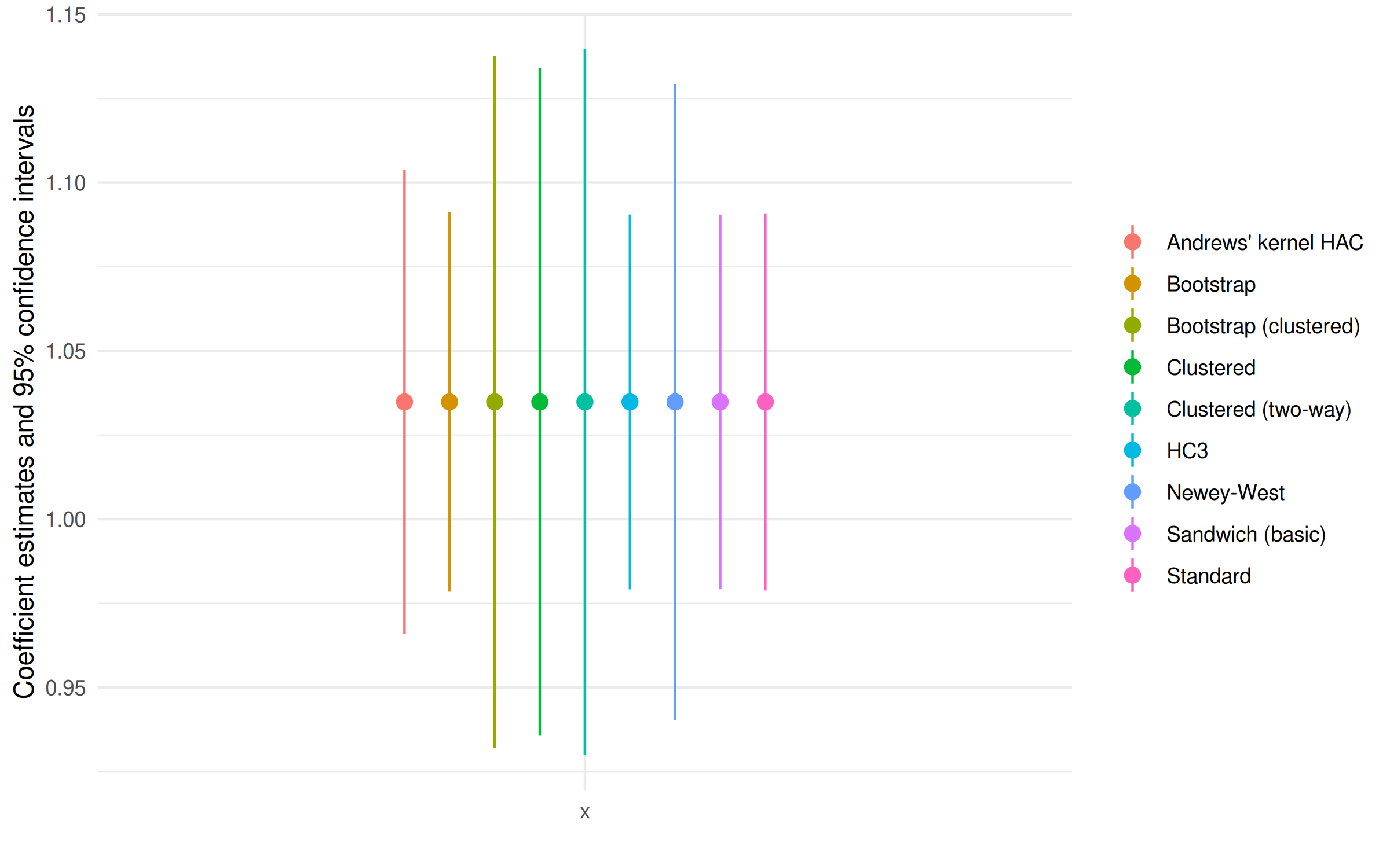
And there you have it: An intuitive and helpful comparison across a host of specifications, even though we only “ran” the underlying model once. Simple!
Example 2: fixest
While sandwich covers a wide range of model classes in R, it’s important to know that a number of libraries provide their own specialised methods for on-the-fly SE adjustment. The one that I want to show you for this second example is the fixest package (@Laurent Bergé).
If you follow me on Twitter or have read my lecture notes, you already know that I am a huge fan of this package. It’s very elegantly designed and provides an insanely fast way to estimate high-dimensional fixed effects models. More importantly for today’s post, fixest offers automatic support for on-the-fly SE adjustment. We only need to run our model once and can then adjust the SEs on the backend via a call to either summary(..., se = 'se_type') or summary(..., cluster = c('cluster_vars').2
To demonstrate, I’m going to run some regressions on a subsample of the well-known RITA air traffic data. I’ve already downloaded the dataset from Revolution Analytics and prepped it for the narrow purposes of this blog post. (See the data appendix below for code.) All told we’re looking at 9 variables extending over approximately 1.8 million rows. So, not “big” data by any stretch of the imagination, but my regressions should take at least a few seconds to run on most computers.
library(data.table)

air = fread('~/air.csv')
air
## year month day_of_week tail_num origin_airport_id dest_airport_id
## 1: 2012 1 3 N320AA 12478 12892
## 2: 2012 1 5 N327AA 12478 12892
## 3: 2012 1 4 N329AA 12892 12478
## 4: 2012 1 5 N336AA 12478 12892
## 5: 2012 1 7 N323AA 12478 12892
## ---
## 1844063: 2011 1 1 N904FJ 14107 15376
## 1844064: 2011 1 1 N7305V 14262 14107
## 1844065: 2011 1 1 N922FJ 14683 11057
## 1844066: 2011 1 1 N935LR 14698 14107
## 1844067: 2011 1 1 N932LR 15376 14107
## arr_delay dep_delay dep_tod
## 1: -34 4 am2
## 2: 2 -2 am2
## 3: -6 -5 am2
## 4: -32 -9 am2
## 5: -7 -6 am2
## ---
## 1844063: -7 -1 pm2
## 1844064: -3 0 pm1
## 1844065: -10 -4 pm2
## 1844066: 11 0 pm1
## 1844067: 30 -5 am2The actual regression that I’m going to run on these data is somewhat uninspired: Namely, how does arrival delay depend on departure delay, conditional on the time of day?3 I’ll throw in a bunch of fixed effects to make the computation a bit more interesting/intensive, but it’s fairly standard stuff. Note that I am running a linear fixed effect model by calling fixest::feols().
But, really, I don’t want you to get sidetrack by the regression details. The main thing I want to focus your attention on is the fact that I’m only going run the base model once, i.e. for mod1. Then, I’m going to adjust the SE for two more models, mod2 and mod3, on the fly via respective summary() calls.
library(fixest)

## Start timer; we'll use for benchmarking later
pt = proc.time()

## Run the model once and once only!
## By default, fixest::feols will cluster the SEs by the first FE (here: month)
mod1 = feols(arr_delay ~ dep_tod / dep_delay |
               month + year + day_of_week + origin_airport_id + dest_airport_id,
             data = air)

## Adjust SEs on the fly: two-way cluster
mod2 = summary(mod1, cluster = c('month', 'origin_airport_id'))

## Adjust SEs on the fly: three-way cluster. Note that we can even include
## cluster vars (e.g. tail_num) that weren't present in the original regression
mod3 = summary(mod1, cluster = c('month', 'origin_airport_id', 'tail_num'))

## Stop timer and save results
time_feols = (proc.time() - pt)[3]
Before I get to benchmarking, how about a quick coefficient plot? I’ll use modelsummary::modelplot() again, focusing only on the key “time of day × departure delay” interaction terms.
feols_mods = list(mod1, mod2, mod3)

modelplot(
  feols_mods,
  coef_map = c('dep_todam1:dep_delay' = 'Midnight × Dep. delay',
               'dep_todam2:dep_delay' = 'Morning × Dep. delay',
               'dep_todpm1:dep_delay' = 'Afternoon × Dep. delay',
               'dep_todpm2:dep_delay' = 'Evening × Dep. delay')
  ) +
  labs(caption = 'Dependent variable: Arrival delay')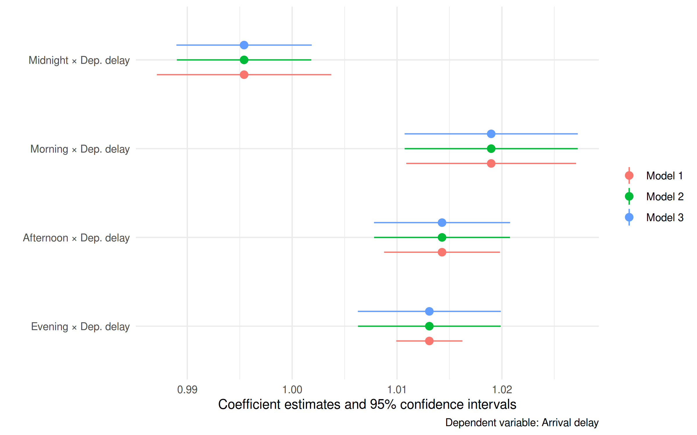
Benchmarking
Great, it worked. But did it save time? To answer this question I’ve benchmarked against three other methods:
feols(), again from the fixest package, but this time with each of the three models run separately.felm()from the lfe package.reghdfefrom the reghdfe package (Stata).
Note: I’m benchmarking against lfe and reghdfe because these two excellent packages have long set the standard for estimating high-dimensional fixed effects models in the social sciences. In other words, I’m trying to convince you of the benefits of on-the-fly SE adjustment by benchmarking against the methods that most people use.
You can find the benchmarking code for these other methods in the appendix. (Please let me know if you spot any errors.) In the interests of brevity, here are the results.
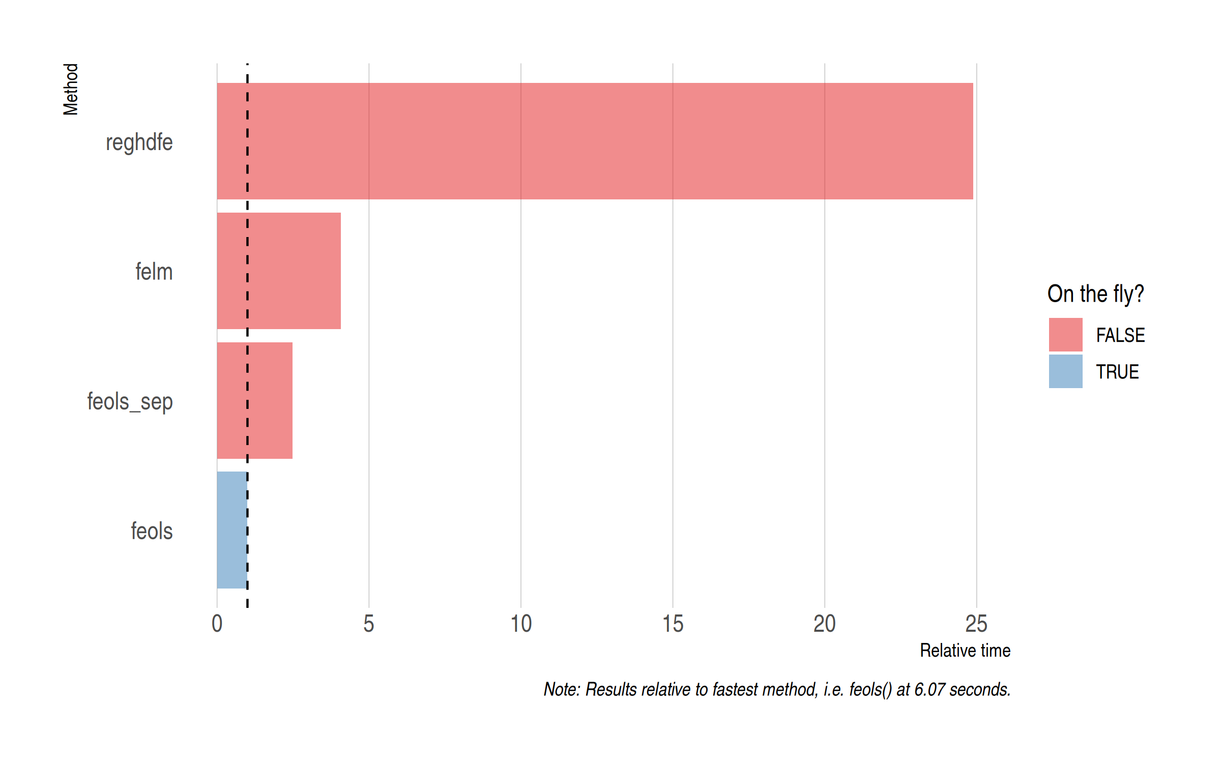
There are several takeaways from this exercise. For example, fixest::feols() is the fastest method even if you are (inefficiently) re-running the models separately. But — yet again and once more, dear friends — the key thing that I want to emphasise is the additional time savings brought on by adjusting the SEs on the fly. Indeed, we can see that the on-the-fly feols approach only takes a third of the time (approximately) that it does to run the models separately. This means that fixest is recomputing the SEs for models 2 and 3 pretty much instantaneously.
To add one last thing about benchmarking, the absolute difference in model run times was not that huge for this particular exercise. There’s maybe two minutes separating the fastest and slowest methods. (Then again, not trivial either…) But if you are like me and find yourself estimating models where each run takes many minutes or hours, or even days and weeks, then the time savings are literally exponential.
Conclusion
There comes a point in almost every empirical project where you have to estimate multiple versions of the same model. Which is to say, the only difference between these multiple versions is how the standard errors were calculated: robust, clustered, etc. Maybe you’re trying to satisfy a referee request before publication. Or, maybe you’re trying to understand how sensitive your results are to different modeling assumptions.
The goal of this blog post has been to show you that there is often a better approach than manually re-running multiple iterations of your model. Instead, I advocate that you run the model once and then adjust your standard errors on the backend, as needed. This “on-the-fly” approach will save you a ton of time if you are working with big datasets. Even if you aren’t working with big data, you will minimize copying and pasting of duplicate code. All of which will help to make your code more readable and cut down on potential errors.
What’s not to like?
P.S. There are a couple of other R libraries with support for on-the-fly SE adjustment, e.g. clubSandwich. Since I’ve used it as a counterfoil in the benchmark, I should add that lfe::felm() provides its own method for swapping out different SEs post-estimation; see here. Similarly, I’ve focused on R because it’s the software language that I use most often and — as far as I am aware — is the only one to provide methods for on-the-fly SE adjustment across a wide range of models. If anyone knows of equivalent methods or canned routines in other languages, please let me know in the comments.
P.P.S. Look, I’m not saying it’s necessarily “wrong” to specify your SEs in the model call. Particularly if you’ve already settled on a single VCOV to use. Then, by all means, use the convenience of Stata’s , robust syntax or the R equivalent lm_robust() (via the estimatr package).
Appendices
Flight data download and prep
if (!file.exists(path.expand('~/air.csv'))) {

  ## Download and extract the data
  URL = 'https://packages.revolutionanalytics.com/datasets/AirlineSubsetCsv.tar.gz'
  dest_file = path.expand('~/AirlineSubsetCsv.tar.gz')
  download.file(URL, dest_file, mode = "wb")
  untar(dest_file, exdir = path.expand('~'))

  ## Bind together and do some data cleaning
  library(data.table)
  csvs = list.files(path.expand('~/AirlineSubsetCsv/'), full.names = TRUE)
  air = rbindlist(lapply(csvs, fread))
  names(air) = tolower(names(air))
  int_vars = c('arr_delay', 'dep_delay', 'dep_time', 'arr_time')
  air[, (int_vars) := lapply(.SD, as.integer), .SDcols = int_vars]

  ## Create a departure 'time of day' factor variable, dividing the day in four
  ## quarters
  air[, dep_tod := fcase(dep_time <= 600, 'am1',
                         dep_time <= 1200, 'am2',
                         dep_time <= 1800, 'pm1',
                         dep_time > 1800, 'pm2')]

  ## Subset
  air = air[!is.na(arr_delay),
            .(year, month, day_of_week, tail_num, origin_airport_id,
              dest_airport_id, arr_delay, dep_delay, dep_tod)]

  ## Write to disk
  fwrite(air, path.expand('~/air.csv'))

  ## Clean up
  file.remove(c(dest_file, csvs))
  file.remove(path.expand('~/AirlineSubsetCsv/')) ## empty dir too
}
Benchmarking code for other methods
fixest (separate models)
# library(fixest) ## Already loaded

pt = proc.time()
mod1a = feols(arr_delay ~ dep_tod / dep_delay |
                month + year + day_of_week + origin_airport_id + dest_airport_id,
              data = air)
mod2a = summary(
  feols(arr_delay ~ dep_tod / dep_delay |
          month + year + day_of_week + origin_airport_id + dest_airport_id,
        data = air),
  cluster = c('month', 'origin_airport_id')
  )
mod3a = summary(
  feols(arr_delay ~ dep_tod / dep_delay |
          month + year + day_of_week + origin_airport_id + dest_airport_id,
        data = air),
  cluster = c('month', 'origin_airport_id', 'tail_num')
  )
time_feols_sep = (proc.time() - pt)[3]
lfe
library(lfe)

pt = proc.time()
est1 = felm(arr_delay ~ dep_tod / dep_delay |
               month + year + day_of_week + origin_airport_id + dest_airport_id |
             0 |
             month,
            data = air)
est2 = felm(arr_delay ~ dep_tod / dep_delay |
               month + year + day_of_week + origin_airport_id + dest_airport_id |
             0 |
             month + origin_airport_id,
            data = air)
est3 = felm(arr_delay ~ dep_tod / dep_delay |
               month + year + day_of_week + origin_airport_id + dest_airport_id |
             0 |
             month + origin_airport_id + tail_num,
            data = air)
time_felm = (proc.time() - pt)[3]
reghdfe
clear
clear matrix
timer clear
set more off

cd "Z:\home\grant"

import delimited air.csv

// Encode strings as numeric factors (Stata struggles with the former)
encode tail_num, generate(tail_num2)
encode dep_tod, generate(dep_tod2)

// Start timer and run regs
timer on 1

qui reghdfe arr_delay i.dep_tod2 i.dep_tod2#c.dep_delay, ///
  absorb(month year day_of_week origin_airport_id dest_airport_id) ///
  cluster(month)

qui reghdfe arr_delay i.dep_tod2 i.dep_tod2#c.dep_delay, ///
  absorb(month year day_of_week origin_airport_id dest_airport_id) ///
  cluster(month origin_airport_id)

qui reghdfe arr_delay i.dep_tod2 i.dep_tod2#c.dep_delay, ///
  absorb(month year day_of_week origin_airport_id dest_airport_id) ///
  cluster(month origin_airport_id tail_num2)

timer off 1

// Export time
drop _all
gen elapsed = .
set obs 1
replace elapsed = r(t1) if _n == 1
outsheet using "reghdfe-ex.csv", replace
-
You can substitute with a regular for loop or
purrr::map()if you prefer. ↩ -
You should read the package documentation for a full description, but very briefly: Valid
searguments are “standard”, “hetero”, “cluster”, “twoway”, “threeway” or “fourway”. Theclusterargument provides an alternative way to be explicit about which variables you want to cluster on. E.g. You would writecluster = c('country', 'year')instead ofse = 'twoway'. ↩ -
Note that I’m going to use a
dep_tod / dep_delayexpansion on the RHS to get the full marginal effect of the interaction terms. Don’t worry too much about this if you haven’t seen it before (click on the previous link if you want to learn more). ↩
Comments