Plot method for emfx objects

Visualize the results of an emfx call.

Usage

# S3 method for class 'emfx'
plot(
  x,
  type = c("pointrange", "errorbar", "ribbon"),
  pch = 16,
  zero = TRUE,
  grid = TRUE,
  ref = -1,
  ...
)

Arguments

x

An emfx object.

type

Character. The type of plot display. One of "pointrange" (default), "errorbar", or "ribbon".

pch

Integer or character. Which plotting character or symbol to use (see points). Defaults to 16 (i.e., small solid circle). Ignored if type = "ribbon".

zero

Logical. Should 0-zero line be emphasized? Default is TRUE.

grid

Logical. Should a background grid be displayed? Default is TRUE.

ref

Integer. Reference line marker for event-study plot. Default is -1 (i.e., the period immediately preceding treatment). To remove completely, set to NA, NULL, or FALSE. Only used if the underlying object was computed using emfx(..., type = "event").

...

Additional arguments passed to tinyplot::tinyplot.

Value

No return value, called for side effect of producing a plot.

Examples

# \dontrun{
# We’ll use the mpdta dataset from the did package (which you’ll need to
# install separately).

# install.packages("did")
data("mpdta", package = "did")

#
# Basic example
#

# The basic ETWFE workflow involves two consecutive function calls:
# 1) `etwfe` and 2) `emfx`

# 1) `etwfe`: Estimate a regression model with saturated interaction terms.
mod = etwfe(
  fml  = lemp ~ lpop, # outcome ~ controls (use 0 or 1 if none)
  tvar = year,        # time variable
  gvar = first.treat, # group variable
  data = mpdta,       # dataset
  vcov = ~countyreal  # vcov adjustment (here: clustered by county)
  )

# mod ## A fixest model object with fully saturated interaction effects.

# 2) `emfx`: Recover the treatment effects of interest.

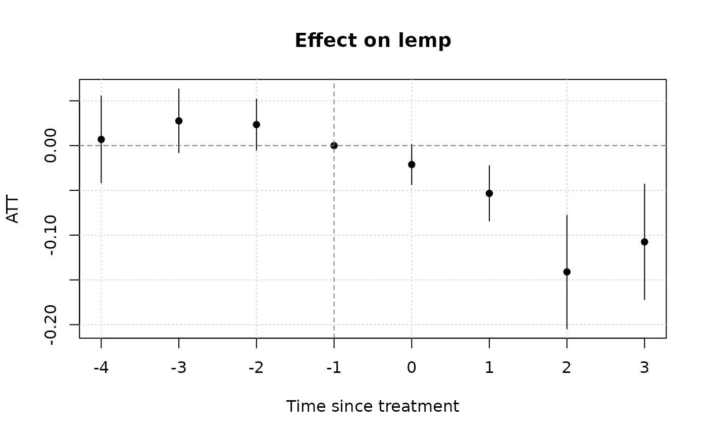
(mod_es = emfx(mod, type = "event")) # dynamic ATE a la an event study
#> 
#>  event Estimate Std. Error     z Pr(>|z|)    S   2.5 %   97.5 %
#>      0  -0.0332     0.0134 -2.48    0.013  6.3 -0.0594 -0.00702
#>      1  -0.0573     0.0171 -3.34   <0.001 10.2 -0.0910 -0.02373
#>      2  -0.1379     0.0308 -4.48   <0.001 17.0 -0.1982 -0.07753
#>      3  -0.1095     0.0323 -3.39   <0.001 10.5 -0.1729 -0.04620
#> 
#> Term: .Dtreat
#> Type: response
#> Comparison: TRUE - FALSE
#> 

# Etc. Other aggregation type options are "simple" (the default), "group"
# and "calendar"

# To visualize results, use the native plot method (see `?plot.emfx`)
plot(mod_es)


# Notice that we don't get any pre-treatment effects with the default
# "notyet" treated control group. Switch to the "never" treated control
# group if you want this.
etwfe(
  lemp ~ lpop, tvar = year, gvar = first.treat, data = mpdta,
  vcov = ~countyreal,
  cgroup = "never"    ## <= use never treated group as control
  ) |>
  emfx("event") |>
  plot()


#
# Heterogeneous treatment effects
#

# Example where we estimate heterogeneous treatment effects for counties
# within the 8 US Great Lake states (versus all other counties).

gls = c("IL" = 17, "IN" = 18, "MI" = 26, "MN" = 27,
        "NY" = 36, "OH" = 39, "PA" = 42, "WI" = 55)

mpdta$gls = substr(mpdta$countyreal, 1, 2) %in% gls

hmod = etwfe(
  lemp ~ lpop, tvar = year, gvar = first.treat, data = mpdta,
  vcov = ~countyreal,
  xvar = gls           ## <= het. TEs by gls
  )

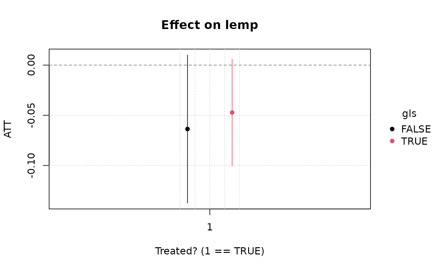
# Heterogeneous ATEs (could also specify "event", etc.)

emfx(hmod)
#> 
#>  .Dtreat   gls Estimate Std. Error     z Pr(>|z|)   S  2.5 %  97.5 %
#>     TRUE FALSE  -0.0637     0.0376 -1.69   0.0905 3.5 -0.137 0.01005
#>     TRUE  TRUE  -0.0472     0.0271 -1.74   0.0816 3.6 -0.100 0.00593
#> 
#> Term: .Dtreat
#> Type: response
#> Comparison: TRUE - FALSE
#> 

# To test whether the ATEs across these two groups (non-GLS vs GLS) are
# statistically different, simply pass an appropriate "hypothesis" argument.

emfx(hmod, hypothesis = "b1 = b2")
#> 
#>  Hypothesis Estimate Std. Error      z Pr(>|z|)   S  2.5 % 97.5 %
#>       b1=b2  -0.0164     0.0558 -0.294    0.768 0.4 -0.126  0.093
#> 
#> Type: response
#> 

plot(emfx(hmod))


#
# Nonlinear model (distribution / link) families
#

# Poisson example

mpdta$emp = exp(mpdta$lemp)

etwfe(
  emp ~ lpop, tvar = year, gvar = first.treat, data = mpdta,
  vcov = ~countyreal,
  family = "poisson"   ## <= family arg for nonlinear options
  ) |>
  emfx("event")
#> The variables '.Dtreat:first.treat::2006:year::2004', '.Dtreat:first.treat::2006:year::2005', '.Dtreat:first.treat::2007:year::2004', '.Dtreat:first.treat::2007:year::2005', '.Dtreat:first.treat::2007:year::2006', '.Dtreat:first.treat::2006:year::2004:lpop_dm' and 4 others have been removed because of collinearity (see $collin.var).
#> 
#>  event Estimate Std. Error       z Pr(>|z|)    S  2.5 % 97.5 %
#>      0   -25.35       15.9 -1.5957  0.11056  3.2  -56.5   5.79
#>      1     1.09       40.3  0.0271  0.97838  0.0  -77.9  80.07
#>      2   -75.12       23.2 -3.2445  0.00118  9.7 -120.5 -29.74
#>      3  -101.82       27.1 -3.7590  < 0.001 12.5 -154.9 -48.73
#> 
#> Term: .Dtreat
#> Type: response
#> Comparison: TRUE - FALSE
#> 
# }