Post-estimation aggregation of ETWFE results

Companion function to etwfe, enabling the recovery of aggregate treatment effects along different dimensions of interest (e.g, an event study of dynamic average treatment effects). emfx is a light wrapper around the slopes function from the marginaleffects package.

Usage

emfx(
  object,
  type = c("simple", "group", "calendar", "event"),
  by_xvar = "auto",
  compress = "auto",
  collapse = compress,
  predict = c("response", "link"),
  post_only = TRUE,
  lean = FALSE,
  ...
)

Arguments

object: An etwfe model object.
type: Character. The desired type of post-estimation aggregation.
by_xvar: Logical. Should the results account for heterogeneous treatment effects? Only relevant if the preceding etwfe call included a specified xvar argument, i.e. interacted categorical covariate. The default behaviour ("auto") is to automatically estimate heterogeneous treatment effects for each level of xvar if these are detected as part of the underlying etwfe model object. Users can override by setting to either FALSE or TRUE. See the "Heterogeneous treatment effects" section below.
compress: Logical. Compress the data by (period by cohort) groups before calculating marginal effects? This trades off a slight loss in precision (typically around the 1st or 2nd significant decimal point) for a substantial improvement in estimation time for large datasets. The default behaviour ("auto") is to automatically compress if the original dataset has more than 500,000 rows. Users can override by setting either FALSE or TRUE. Note that collapsing by group is only valid if the preceding etwfe call was run with "ivar = NULL" (the default). See the "Performance tips" section below.
collapse: Logical. An alias for compress (only used for backwards compatability and ignored if both arguments are provided). The behaviour is identical, but it will trigger a message nudging users to rather use the compress argument.
predict: Character. The type (scale) of prediction used to compute the marginal effects. If "response" (the default), then the output is at the level of the response variable, i.e. it is the expected predictor \(E(Y|X)\). If "link", the value returned is the linear predictor of the fitted model, i.e. \(X\cdot \beta\). The difference should only matter for nonlinear models. (Note: This argument is typically called type when use in predict or slopes, but we rename it here to avoid a clash with the top-level type argument above.)
post_only: Logical. Drop pre-treatment ATTs? Only evaluated if (a) type = "event" and (b) the original etwfe model object was estimated using the default "notyet" treated control group. If conditions (a) and (b) are met then the pre-treatment effects will be zero as a mechanical result of ETWFE's estimation setup. The default behaviour (TRUE) is thus to drop these nuisance rows from the dataset. The post_only argument recognises that you may still want to keep them for presentation purposes (e.g., plotting an event study). Nevertheless, be forewarned that enabling that behaviour via FALSE is strictly performative: the "zero" treatment effects for any pre-treatment periods is purely an artefact of the estimation setup.
lean: Logical. Default is FALSE. Switching to TRUE enforces a lean return object; namely a simple data.frame of the main results, stripped of ancillary attributes. Note that this will disable some advanced marginaleffects post-processing features, but those are unlikely to be used in the emfx context. The upside is a potentially dramatic reduction in the size of the return object. Consequently, we may change the default to TRUE in a future version of etwfe.
...: Additional arguments passed to marginaleffects::slopes. For example, you can pass vcov = FALSE to dramatically speed up estimation times of the main marginal effects (but at the cost of not getting any information about standard errors; see Performance tips below). Another potentially useful application is testing whether heterogeneous treatment effects (i.e., the levels of any xvar covariate) are equal by invoking the hypothesis argument, e.g. hypothesis = "b1 = b2".

Value

A data.frame of aggregated treatment effects along the dimension(s) of interested. Note that this data.frame will have been overloaded with the slopes class, and so will come with a special print method. But the underlying columns will usually include:

term
contrast
<type> (i.e., the name of your type string)
estimate
std.error
statistic
p.value
s.value
conf.low
conf.high

Performance tips

Under most situations, etwfe should complete very quickly. For its part, emfx is quite performant too and should take a few seconds or less for datasets under 100k rows. However, emfx's computation time does tend to scale non-linearly with the size of the original data, as well as the number of interactions from the underlying etwfe model. Without getting too deep into the weeds, the numerical delta method used to recover the ATEs of interest has to estimate two prediction models for each coefficient in the model and then compute their standard errors. So, it's a potentially expensive operation that can push the computation time for large datasets (> 1m rows) up to several minutes or longer.

Fortunately, there are two complementary strategies that you can use to speed things up. The first is to turn off the most expensive part of the whole procedure—standard error calculation—by calling emfx(..., vcov = FALSE). Doing so should bring the estimation time back down to a few seconds or less, even for datasets in excess of a million rows. While the loss of standard errors might not be an acceptable trade-off for projects where statistical inference is critical, the good news is this first strategy can still be combined our second strategy. It turns out that collapsing the data by groups prior to estimating the marginal effects can yield substantial speed gains of its own. Users can do this by invoking the emfx(..., collapse = TRUE) argument. While the effect here is not as dramatic as the first strategy, our second strategy does have the virtue of retaining information about the standard errors. The trade-off this time, however, is that collapsing our data does lead to a loss in accuracy for our estimated parameters. On the other hand, testing suggests that this loss in accuracy tends to be relatively minor, with results equivalent up to the 1st or 2nd significant decimal place (or even better).

Summarizing, here's a quick plan of attack for you to try if you are worried about the estimation time for large datasets and models:

Estimate mod = etwfe(...) as per usual.
Run emfx(mod, vcov = FALSE, ...).
Run emfx(mod, vcov = FALSE, collapse = TRUE, ...).
Compare the point estimates from steps 1 and 2. If they are are similar enough to your satisfaction, get the approximate standard errors by running emfx(mod, collapse = TRUE, ...).

Heterogeneous treatment effects

Specifying etwfe(..., xvar = <xvar>) will generate interaction effects for all levels of <xvar> as part of the main regression model. The reason that this is useful (as opposed to a regular, non-interacted covariate in the formula RHS) is that it allows us to estimate heterogeneous treatment effects as part of the larger ETWFE framework. Specifically, we can recover heterogeneous treatment effects for each level of <xvar> by passing the resulting etwfe model object on to emfx().

For example, imagine that we have a categorical variable called "age" in our dataset, with two distinct levels "adult" and "child". Running emfx(etwfe(..., xvar = age)) will tell us how the efficacy of treatment varies across adults and children. We can then also leverage the in-built hypothesis testing infrastructure of marginaleffects to test whether the treatment effect is statistically different across these two age groups; see Examples below. Note the same principles carry over to categorical variables with multiple levels, or even continuous variables (although continuous variables are not as well supported yet).

References

Wong, Jeffrey et al. (2021). You Only Compress Once: Optimal Data Compression for Estimating Linear Models. Working paper (version: March 16, 2021). Available: https://doi.org/10.48550/arXiv.2102.11297

Examples

# \dontrun{
# We’ll use the mpdta dataset from the did package (which you’ll need to 
# install separately).

# install.packages("did")
data("mpdta", package = "did")

#
# Basic example
#

# The basic ETWFE workflow involves two consecutive function calls:
# 1) `etwfe` and 2) `emfx`

# 1) `etwfe`: Estimate a regression model with saturated interaction terms.
mod = etwfe(
  fml  = lemp ~ lpop, # outcome ~ controls (use 0 or 1 if none)
  tvar = year,        # time variable
  gvar = first.treat, # group variable
  data = mpdta,       # dataset
  vcov = ~countyreal  # vcov adjustment (here: clustered by county)
  )

# mod ## A fixest model object with fully saturated interaction effects.

# 2) `emfx`: Recover the treatment effects of interest.

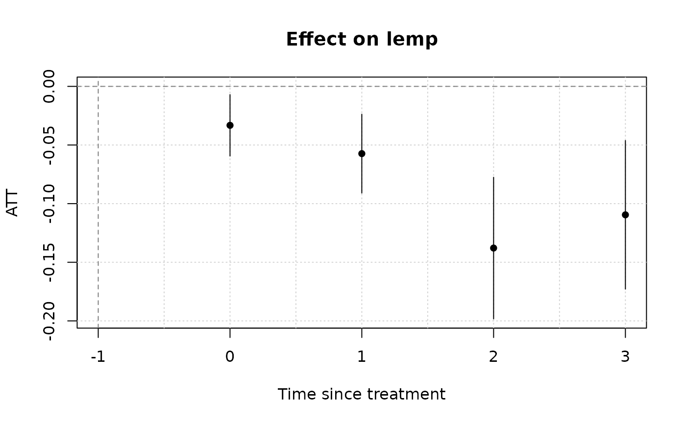
(mod_es = emfx(mod, type = "event")) # dynamic ATE a la an event study
#> 
#>     Term event Estimate Std. Error     z Pr(>|z|)    S   2.5 %   97.5 %
#>  .Dtreat     0  -0.0332     0.0134 -2.48    0.013  6.3 -0.0594 -0.00701
#>  .Dtreat     1  -0.0573     0.0172 -3.34   <0.001 10.2 -0.0910 -0.02373
#>  .Dtreat     2  -0.1379     0.0308 -4.48   <0.001 17.0 -0.1982 -0.07751
#>  .Dtreat     3  -0.1095     0.0323 -3.39   <0.001 10.5 -0.1729 -0.04619
#> 
#> Type:  response 
#> Comparison: TRUE - FALSE
#> Columns: term, contrast, event, estimate, std.error, statistic, p.value, s.value, conf.low, conf.high 
#> 

# Etc. Other aggregation type options are "simple" (the default), "group"
# and "calendar"

# To visualize results, use the native plot method (see `?plot.emfx`)
plot(mod_es)


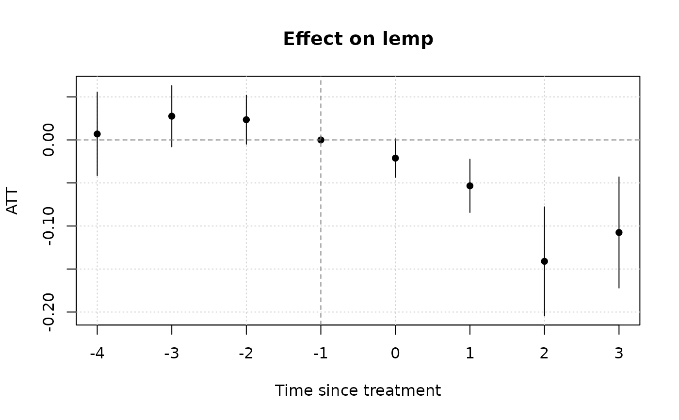
# Notice that we don't get any pre-treatment effects with the default
# "notyet" treated control group. Switch to the "never" treated control
# group if you want this.
etwfe(
  lemp ~ lpop, tvar = year, gvar = first.treat, data = mpdta,
  vcov = ~countyreal,
  cgroup = "never"    ## <= use never treated group as control
  ) |>
  emfx("event") |>
  plot()


#
# Heterogeneous treatment effects
#

# Example where we estimate heterogeneous treatment effects for counties 
# within the 8 US Great Lake states (versus all other counties). 

gls = c("IL" = 17, "IN" = 18, "MI" = 26, "MN" = 27,
        "NY" = 36, "OH" = 39, "PA" = 42, "WI" = 55)

mpdta$gls = substr(mpdta$countyreal, 1, 2) %in% gls

hmod = etwfe(
  lemp ~ lpop, tvar = year, gvar = first.treat, data = mpdta, 
  vcov = ~countyreal,
  xvar = gls           ## <= het. TEs by gls
  )

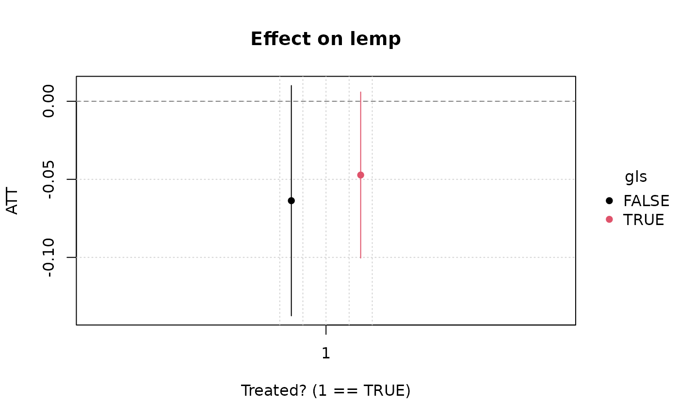
# Heterogeneous ATEs (could also specify "event", etc.) 

emfx(hmod)
#> 
#>     Term .Dtreat   gls Estimate Std. Error     z Pr(>|z|)   S  2.5 %  97.5 %
#>  .Dtreat    TRUE FALSE  -0.0637     0.0376 -1.69   0.0906 3.5 -0.137 0.01007
#>  .Dtreat    TRUE  TRUE  -0.0472     0.0271 -1.74   0.0817 3.6 -0.100 0.00594
#> 
#> Type:  response 
#> Comparison: TRUE - FALSE
#> Columns: term, contrast, .Dtreat, gls, estimate, std.error, statistic, p.value, s.value, conf.low, conf.high 
#> 

# To test whether the ATEs across these two groups (non-GLS vs GLS) are 
# statistically different, simply pass an appropriate "hypothesis" argument.

emfx(hmod, hypothesis = "b1 = b2")
#> Warning: 
#> It is essential to check the order of estimates when specifying hypothesis tests using positional indices like b1, b2, etc. The indices of estimates can change depending on the order of rows in the original dataset, user-supplied arguments, model-fitting package, and version of `marginaleffects`. 
#> 
#> It is also good practice to use assertions that ensure the order of estimates is consistent across different runs of the same code. Example:
#> 
#> ```r
#> mod <- lm(mpg ~ am * carb, data = mtcars)
#> 
#> # assertion for safety
#> p <- avg_predictions(mod, by = 'carb')
#> stopifnot(p$carb[1] != 1 || p$carb[2] != 2)
#> 
#> # hypothesis test
#> avg_predictions(mod, by = 'carb', hypothesis = 'b1 - b2 = 0')
#> ```
#> 
#> Disable this warning with: `options(marginaleffects_safe = FALSE)`
#> This warning appears once per session.
#> 
#>   Term Estimate Std. Error      z Pr(>|z|)   S  2.5 % 97.5 %
#>  b1=b2  -0.0164     0.0559 -0.294    0.769 0.4 -0.126  0.093
#> 
#> Type:  response 
#> Columns: term, estimate, std.error, statistic, p.value, s.value, conf.low, conf.high 
#> 

plot(emfx(hmod))


#
# Nonlinear model (distribution / link) families
#

# Poisson example

mpdta$emp = exp(mpdta$lemp)

etwfe(
  emp ~ lpop, tvar = year, gvar = first.treat, data = mpdta, 
  vcov = ~countyreal,
  family = "poisson"   ## <= family arg for nonlinear options
  ) |>
  emfx("event")
#> The variables '.Dtreat:first.treat::2006:year::2004', '.Dtreat:first.treat::2006:year::2005', '.Dtreat:first.treat::2007:year::2004', '.Dtreat:first.treat::2007:year::2005', '.Dtreat:first.treat::2007:year::2006', '.Dtreat:first.treat::2006:year::2004:lpop_dm' and 4 others have been removed because of collinearity (see $collin.var).
#> 
#>     Term event Estimate Std. Error       z Pr(>|z|)    S  2.5 % 97.5 %
#>  .Dtreat     0   -25.35       15.9 -1.5942    0.111  3.2  -56.5   5.82
#>  .Dtreat     1     1.09       41.8  0.0261    0.979  0.0  -80.9  83.09
#>  .Dtreat     2   -75.12       22.3 -3.3696   <0.001 10.4 -118.8 -31.43
#>  .Dtreat     3  -101.82       28.1 -3.6234   <0.001 11.7 -156.9 -46.75
#> 
#> Type:  response 
#> Comparison: TRUE - FALSE
#> Columns: term, contrast, event, estimate, std.error, statistic, p.value, s.value, conf.low, conf.high 
#> 
# }