Extended two-way fixed effects

Estimates an "extended" two-way fixed effects regression, with fully saturated interaction effects a la Wooldridge (2021, 2023). At its heart, etwfe is a convenience function that automates a number of tedious and error prone preparation steps involving both the data and model formulae. Computation is passed on to the feols (linear) / feglm (nonlinear) functions from the fixest package. etwfe should be paired with its companion emfx function.

Usage

etwfe(
  fml = NULL,
  tvar = NULL,
  gvar = NULL,
  data = NULL,
  ivar = NULL,
  xvar = NULL,
  tref = NULL,
  gref = NULL,
  cgroup = c("notyet", "never"),
  fe = c("vs", "feo", "none"),
  family = NULL,
  ...
)

Arguments

fml: A two-side formula representing the outcome (lhs) and any control variables (rhs), e.g. y ~ x1 + x2. If no controls are required, the rhs must take the value of 0 or 1, e.g. y ~ 0.
tvar: Time variable. Can be a string (e.g., "year") or an expression (e.g., year).
gvar: Group variable. Can be either a string (e.g., "first_treated") or an expression (e.g., first_treated). In a staggered treatment setting, the group variable typically denotes treatment cohort.
data: The data frame that you want to run ETWFE on.
ivar: Optional index variable. Can be a string (e.g., "country") or an expression (e.g., country). Leaving as NULL (the default) will result in group-level fixed effects being used, which is more efficient and necessary for nonlinear models (see family argument below). However, you may still want to cluster your standard errors by your index variable through the vcov argument. See Examples below.
xvar: Optional interacted categorical covariate for estimating heterogeneous treatment effects. Enables recovery of the marginal treatment effect for distinct levels of xvar, e.g. "child", "teenager", or "adult". Note that the "x" prefix in "xvar" represents a covariate that is interacted with treatment, as opposed to a regular control variable.
tref: Optional reference value for tvar. Defaults to its minimum value (i.e., the first time period observed in the dataset).
gref: Optional reference value for gvar. You shouldn't need to provide this if your gvar variable is well specified. But providing an explicit reference value can be useful/necessary if the desired control group takes an unusual value.
cgroup: What control group do you wish to use for estimating treatment effects. Either "notyet" treated (the default) or "never" treated.
fe: What level of fixed effects should be used? Defaults to "vs" (varying slopes), which is the most efficient in terms of estimation and terseness of the return model object. The other two options, "feo" (fixed effects only) and "none" (no fixed effects whatsoever), trade off efficiency for additional information on other (nuisance) model parameters. Note that the primary treatment parameters of interest should remain unchanged regardless of choice.
family: Which family to use for the estimation. Defaults to NULL, in which case fixest::feols is used. Otherwise passed to fixest::feglm, so that valid entries include "logit", "poisson", and "negbin". Note that if a non-NULL family entry is detected, ivar will automatically be set to NULL.
...: Additional arguments passed to fixest::feols (or fixest::feglm). The most common example would be a vcov argument.

Value

A fixest object with fully saturated interaction effects, and a few additional attributes used for post-estimation in emfx.

Heterogeneous treatment effects

Specifying etwfe(..., xvar = <xvar>) will generate interaction effects for all levels of <xvar> as part of the main regression model. The reason that this is useful (as opposed to a regular, non-interacted covariate in the formula RHS) is that it allows us to estimate heterogeneous treatment effects as part of the larger ETWFE framework. Specifically, we can recover heterogeneous treatment effects for each level of <xvar> by passing the resulting etwfe model object on to emfx().

For example, imagine that we have a categorical variable called "age" in our dataset, with two distinct levels "adult" and "child". Running emfx(etwfe(..., xvar = age)) will tell us how the efficacy of treatment varies across adults and children. We can then also leverage the in-built hypothesis testing infrastructure of marginaleffects to test whether the treatment effect is statistically different across these two age groups; see Examples below. Note the same principles carry over to categorical variables with multiple levels, or even continuous variables (although continuous variables are not as well supported yet).

Performance tips

Under most situations, etwfe should complete very quickly. For its part, emfx is quite performant too and should take a few seconds or less for datasets under 100k rows. However, emfx's computation time does tend to scale non-linearly with the size of the original data, as well as the number of interactions from the underlying etwfe model. Without getting too deep into the weeds, the numerical delta method used to recover the ATEs of interest has to estimate two prediction models for each coefficient in the model and then compute their standard errors. So, it's a potentially expensive operation that can push the computation time for large datasets (> 1m rows) up to several minutes or longer.

Fortunately, there are two complementary strategies that you can use to speed things up. The first is to turn off the most expensive part of the whole procedure—standard error calculation—by calling emfx(..., vcov = FALSE). Doing so should bring the estimation time back down to a few seconds or less, even for datasets in excess of a million rows. While the loss of standard errors might not be an acceptable trade-off for projects where statistical inference is critical, the good news is this first strategy can still be combined our second strategy. It turns out that collapsing the data by groups prior to estimating the marginal effects can yield substantial speed gains of its own. Users can do this by invoking the emfx(..., collapse = TRUE) argument. While the effect here is not as dramatic as the first strategy, our second strategy does have the virtue of retaining information about the standard errors. The trade-off this time, however, is that collapsing our data does lead to a loss in accuracy for our estimated parameters. On the other hand, testing suggests that this loss in accuracy tends to be relatively minor, with results equivalent up to the 1st or 2nd significant decimal place (or even better).

Summarizing, here's a quick plan of attack for you to try if you are worried about the estimation time for large datasets and models:

Estimate mod = etwfe(...) as per usual.
Run emfx(mod, vcov = FALSE, ...).
Run emfx(mod, vcov = FALSE, collapse = TRUE, ...).
Compare the point estimates from steps 1 and 2. If they are are similar enough to your satisfaction, get the approximate standard errors by running emfx(mod, collapse = TRUE, ...).

References

Wooldridge, Jeffrey M. (2021). Two-Way Fixed Effects, the Two-Way Mundlak Regression, and Difference-in-Differences Estimators. Working paper (version: August 16, 2021). Available: http://dx.doi.org/10.2139/ssrn.3906345

Wooldridge, Jeffrey M. (2023). Simple Approaches to Nonlinear Difference-in-Differences with Panel Data. The Econometrics Journal, 26(3), C31-C66. Available: https://doi.org/10.1093/ectj/utad016

Examples

# \dontrun{
# We’ll use the mpdta dataset from the did package (which you’ll need to 
# install separately).

# install.packages("did")
data("mpdta", package = "did")

#
# Basic example
#

# The basic ETWFE workflow involves two consecutive function calls:
# 1) `etwfe` and 2) `emfx`

# 1) `etwfe`: Estimate a regression model with saturated interaction terms.
mod = etwfe(
  fml  = lemp ~ lpop, # outcome ~ controls (use 0 or 1 if none)
  tvar = year,        # time variable
  gvar = first.treat, # group variable
  data = mpdta,       # dataset
  vcov = ~countyreal  # vcov adjustment (here: clustered by county)
  )

# mod ## A fixest model object with fully saturated interaction effects.

# 2) `emfx`: Recover the treatment effects of interest.

(mod_es = emfx(mod, type = "event")) # dynamic ATE a la an event study
#> 
#>  event Estimate Std. Error     z Pr(>|z|)    S   2.5 %   97.5 %
#>      0  -0.0332     0.0134 -2.48    0.013  6.3 -0.0594 -0.00701
#>      1  -0.0573     0.0172 -3.34   <0.001 10.2 -0.0910 -0.02373
#>      2  -0.1379     0.0308 -4.48   <0.001 17.0 -0.1982 -0.07751
#>      3  -0.1095     0.0323 -3.39   <0.001 10.5 -0.1729 -0.04619
#> 
#> Term: .Dtreat
#> Type:  response 
#> Comparison: TRUE - FALSE
#> 

# Etc. Other aggregation type options are "simple" (the default), "group"
# and "calendar"

# To visualize results, use the native plot method (see `?plot.emfx`)
plot(mod_es)


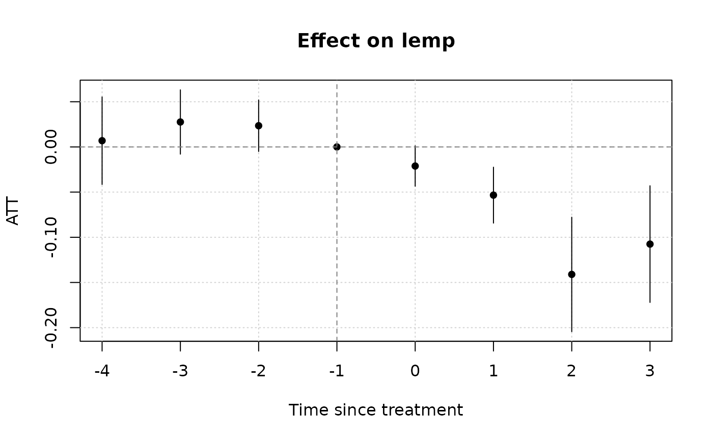
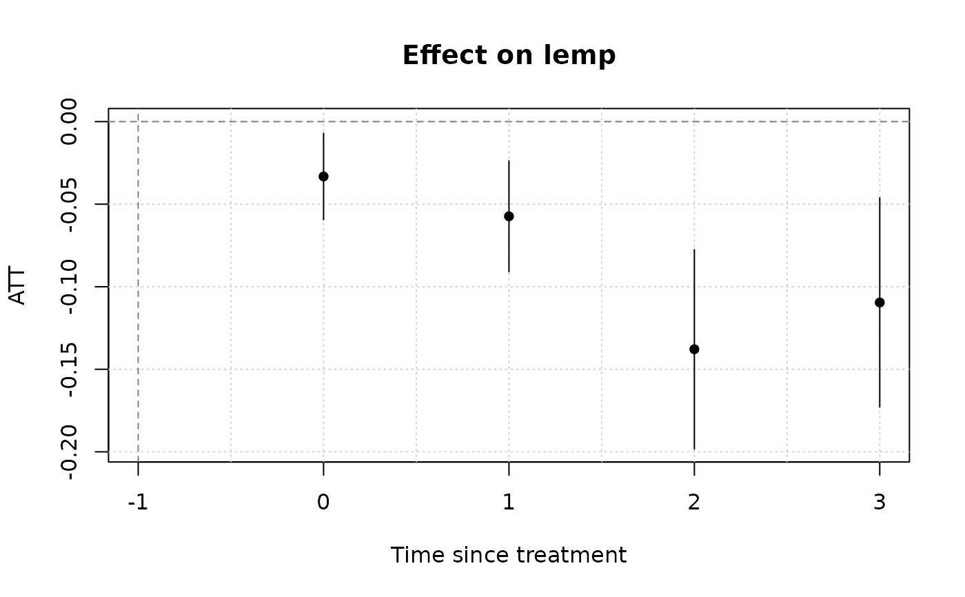# Notice that we don't get any pre-treatment effects with the default
# "notyet" treated control group. Switch to the "never" treated control
# group if you want this.
etwfe(
  lemp ~ lpop, tvar = year, gvar = first.treat, data = mpdta,
  vcov = ~countyreal,
  cgroup = "never"    ## <= use never treated group as control
  ) |>
  emfx("event") |>
  plot()


#
# Heterogeneous treatment effects
#

# Example where we estimate heterogeneous treatment effects for counties 
# within the 8 US Great Lake states (versus all other counties). 

gls = c("IL" = 17, "IN" = 18, "MI" = 26, "MN" = 27,
        "NY" = 36, "OH" = 39, "PA" = 42, "WI" = 55)

mpdta$gls = substr(mpdta$countyreal, 1, 2) %in% gls

hmod = etwfe(
  lemp ~ lpop, tvar = year, gvar = first.treat, data = mpdta, 
  vcov = ~countyreal,
  xvar = gls           ## <= het. TEs by gls
  )

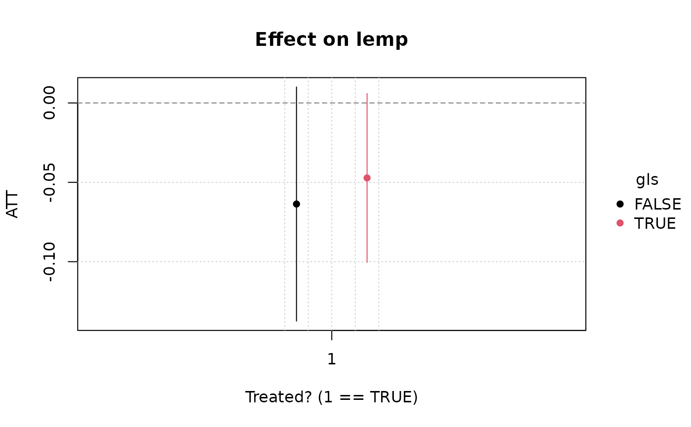
# Heterogeneous ATEs (could also specify "event", etc.) 

emfx(hmod)
#> 
#>  .Dtreat   gls Estimate Std. Error     z Pr(>|z|)   S  2.5 %  97.5 %
#>     TRUE FALSE  -0.0637     0.0376 -1.69   0.0906 3.5 -0.137 0.01007
#>     TRUE  TRUE  -0.0472     0.0271 -1.74   0.0817 3.6 -0.100 0.00594
#> 
#> Term: .Dtreat
#> Type:  response 
#> Comparison: TRUE - FALSE
#> 

# To test whether the ATEs across these two groups (non-GLS vs GLS) are 
# statistically different, simply pass an appropriate "hypothesis" argument.

emfx(hmod, hypothesis = "b1 = b2")
#> 
#>  Hypothesis Estimate Std. Error      z Pr(>|z|)   S  2.5 % 97.5 %
#>       b1=b2  -0.0164     0.0559 -0.294    0.769 0.4 -0.126  0.093
#> 
#> Type:  response 
#> 

plot(emfx(hmod))


#
# Nonlinear model (distribution / link) families
#

# Poisson example

mpdta$emp = exp(mpdta$lemp)

etwfe(
  emp ~ lpop, tvar = year, gvar = first.treat, data = mpdta, 
  vcov = ~countyreal,
  family = "poisson"   ## <= family arg for nonlinear options
  ) |>
  emfx("event")
#> The variables '.Dtreat:first.treat::2006:year::2004', '.Dtreat:first.treat::2006:year::2005', '.Dtreat:first.treat::2007:year::2004', '.Dtreat:first.treat::2007:year::2005', '.Dtreat:first.treat::2007:year::2006', '.Dtreat:first.treat::2006:year::2004:lpop_dm' and 4 others have been removed because of collinearity (see $collin.var).
#> 
#>  event Estimate Std. Error       z Pr(>|z|)    S  2.5 % 97.5 %
#>      0   -25.35       15.9 -1.5942    0.111  3.2  -56.5   5.82
#>      1     1.09       41.8  0.0261    0.979  0.0  -80.9  83.09
#>      2   -75.12       22.3 -3.3696   <0.001 10.4 -118.8 -31.43
#>      3  -101.82       28.1 -3.6234   <0.001 11.7 -156.9 -46.75
#> 
#> Term: .Dtreat
#> Type:  response 
#> Comparison: TRUE - FALSE
#> 
# }

References

Wooldridge, Jeffrey M. (2025). Two-way fixed effects, the two-way Mundlak regression, and difference-in-differences estimators. Empirical Economics, 69, 2545-2587. Available: https://doi.org/10.1007/s00181-025-02807-z