Convert a decision tree into a data frame of partition coordinates

Extracts the terminal leaf nodes of a decision tree that contains no more that two numeric predictor variables. These leaf nodes are then converted into a data frame, where each row represents a partition (or leaf or terminal node) that can easily be plotted in 2-D coordinate space.

Usage

parttree(tree, keep_as_dt = FALSE, flip = FALSE)

Arguments

tree

An rpart.object or alike. This includes compatible classes from the mlr3 and tidymodels frontends, or the constparty class inheriting from party.

keep_as_dt

Logical. The function relies on data.table for internal data manipulation. But it will coerce the final return object into a regular data frame (default behavior) unless the user specifies TRUE.

flip

Logical. Should we flip the "x" and "y" variables in the return data frame? The default behaviour is for the first split variable in the tree to take the "y" slot, and any second split variable to take the "x" slot. Setting to TRUE switches these around.

Note: This argument is primarily useful when it passed via geom_parttree to ensure correct axes orientation as part of a ggplot2 visualization (see geom_parttree Examples). We do not expect users to call parttree(..., flip = TRUE) directly. Similarly, to switch axes orientation for the native (base graphics) plot.parttree method, we recommend calling plot(..., flip = TRUE) rather than flipping the underlying parttree object.

Value

A data frame comprising seven columns: the leaf node, its path, a set of rectangle limits (i.e., xmin, xmax, ymin, ymax), and a final column corresponding to the predicted value for that leaf.

See also

plot.parttree, geom_parttree, rpart, ctree partykit::ctree.

Examples

library("parttree")
#
## rpart trees

library("rpart")
rp = rpart(Kyphosis ~ Start + Age, data = kyphosis)

# A parttree object is just a data frame with additional attributes
(rp_pt = parttree(rp))
#>   node Kyphosis                                                       path xmin
#> 1    3  present                                                Start < 8.5 -Inf
#> 2    4   absent                             Start >= 8.5 --> Start >= 14.5 14.5
#> 3   10   absent                 Start >= 8.5 --> Start < 14.5 --> Age < 55  8.5
#> 4   22   absent Start >= 8.5 --> Start < 14.5 --> Age >= 55 --> Age >= 111  8.5
#> 5   23  present  Start >= 8.5 --> Start < 14.5 --> Age >= 55 --> Age < 111  8.5
#>   xmax ymin ymax
#> 1  8.5 -Inf  Inf
#> 2  Inf -Inf  Inf
#> 3 14.5 -Inf   55
#> 4 14.5  111  Inf
#> 5 14.5   55  111
attr(rp_pt, "parttree")
#> $xvar
#> [1] "Start"
#> 
#> $yvar
#> [1] "Age"
#> 
#> $xrange
#> [1]  1 18
#> 
#> $yrange
#> [1]   1 206
#> 
#> $response
#> [1] "Kyphosis"
#> 
#> $call
#> rpart(formula = Kyphosis ~ Start + Age, data = kyphosis)
#> 
#> $na.action
#> NULL
#> 
#> $flip
#> [1] FALSE
#> 
#> $raw_data
#> NULL
#> 

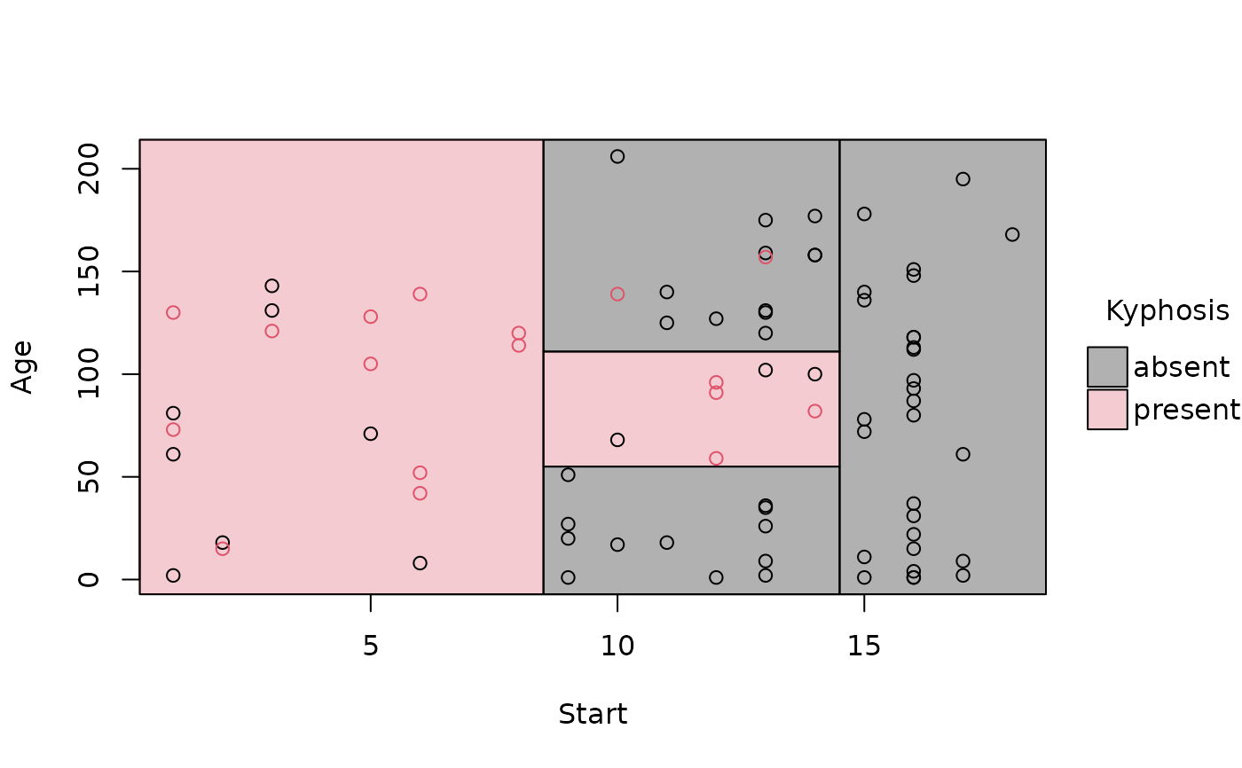
# simple plot
plot(rp_pt)


# removing the (recursive) partition borders helps to emphasise overall fit
plot(rp_pt, border = NA)


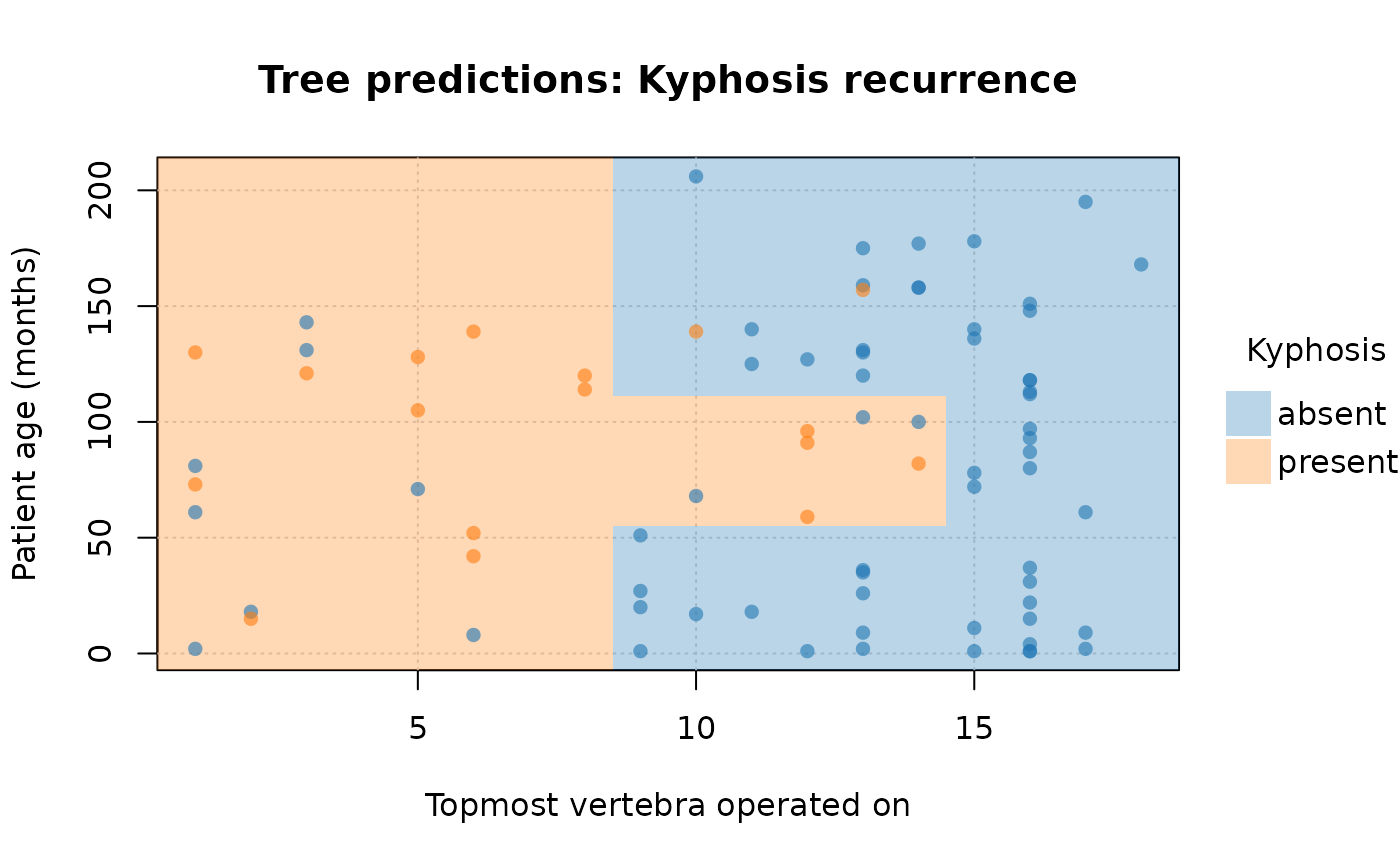
# customize further by passing extra options to (tiny)plot
plot(
   rp_pt,
   border  = NA,                                     # no partition borders
   pch     = 16,                                     # filled points
   alpha   = 0.6,                                    # point transparency
   grid    = TRUE,                                   # background grid
   palette = "classic",                              # new colour palette
   xlab    = "Topmost vertebra operated on",         # custom x title
   ylab    = "Patient age (months)",                 # custom y title
   main    = "Tree predictions: Kyphosis recurrence" # custom title
)


#
## conditional inference trees from partyit

library("partykit")
#> Loading required package: grid
#> Loading required package: libcoin
#> Loading required package: mvtnorm
ct = ctree(Species ~ Petal.Length + Petal.Width, data = iris)
ct_pt = parttree(ct)
plot(ct_pt, pch = 19, palette = "okabe", main = "ctree predictions: iris species")
#> Error in eval(raw_data): object 'ct' not found

## rpart via partykit
rp2 = as.party(rp)
parttree(rp2)
#>   node Kyphosis                                                       path xmin
#> 3    3   absent                               Start < 8.5 --> Start < 14.5 14.5
#> 5    5   absent                 Start < 8.5 --> Start >= 14.5 --> Age < 55  8.5
#> 7    7   absent  Start < 8.5 --> Start >= 14.5 --> Age >= 55 --> Age < 111  8.5
#> 8    8  present Start < 8.5 --> Start >= 14.5 --> Age >= 55 --> Age >= 111  8.5
#> 9    9  present                                               Start >= 8.5 -Inf
#>   xmax ymin ymax
#> 3  Inf -Inf  Inf
#> 5 14.5 -Inf   55
#> 7 14.5  111  Inf
#> 8 14.5   55  111
#> 9  8.5 -Inf  Inf

#
## various front-end frameworks are also supported, e.g.

# tidymodels

# install.packages("parsnip")
library(parsnip)

decision_tree() |>
  set_engine("rpart") |>
  set_mode("classification") |>
  fit(Species ~ Petal.Length + Petal.Width, data=iris) |>
  parttree() |>
  plot(main = "This time brought to you via parsnip...")


# mlr3 (NB: use `keep_model = TRUE` for mlr3 learners)

# install.packages("mlr3")
library(mlr3)

task_iris = TaskClassif$new("iris", iris, target = "Species")
task_iris$formula(rhs = "Petal.Length + Petal.Width")
#> Species ~ `Petal.Length + Petal.Width`
#> NULL
fit_iris = lrn("classif.rpart", keep_model = TRUE) # NB!
fit_iris$train(task_iris)
plot(parttree(fit_iris), main = "... and now mlr3")