import polars as pl
import time
import matplotlibPolars from Python and R
Pro-tip: Just swap . (Python) for $ (R), or vice versa
Load libraries
library(polars)Scan data
nyc = pl.scan_parquet("nyc-taxi/**/*.parquet", hive_partitioning=True)
nyc
NAIVE QUERY PLAN
run LazyFrame.show_graph() to see the optimized version
nyc = pl$scan_parquet("nyc-taxi/**/*.parquet", hive_partitioning=TRUE)
nyc<polars_lazy_frame>First example
Polars operations are registered as queries until they are collected.
q1 = (
    nyc
    .group_by(["passenger_count"])
    .agg([
            pl.mean("tip_amount")#.alias("mean_tip") ## alias is optional
        ])
    .sort("passenger_count")
)
q1
NAIVE QUERY PLAN
run LazyFrame.show_graph() to see the optimized version
q1 = (
    nyc
    $group_by("passenger_count")
    $agg(
        pl$col("tip_amount")$mean()#$alias("mean_tip") ## alias is optional
    )
    $sort("passenger_count")
)
q1
<polars_lazy_frame>
NoteR-polars multiline syntax
Polars-style x$method1()$method2()... chaining may seem a little odd to R users, especially for multiline queries. Here I have adopted the same general styling as Python: By enclosing the full query in parentheses (), we can start each $method() on a new line. If this isn’t to your fancy, you could also rewrite these multiline queries as follows:
nyc$group_by(
    "passenger_count"
)$agg(
    pl$col("tip_amount")$mean()
)$sort("passenger_count")
(Note: this is the naive query plan, not the optimized query that polars will actually implement for us. We’ll come back to this idea shortly.)
Calling collect() enforces computation.
tic = time.time()
dat1 = q1.collect()
toc = time.time()

dat1
shape: (18, 2)
| passenger_count | tip_amount |
|---|---|
| i64 | f64 |
| 0 | 0.862099 |
| 1 | 1.151011 |
| 2 | 1.08158 |
| 3 | 0.962949 |
| 4 | 0.844519 |
| … | … |
| 177 | 1.0 |
| 208 | 0.0 |
| 247 | 2.3 |
| 249 | 0.0 |
| 254 | 0.0 |
# print(f"Time difference of {toc - tic} seconds")tic = Sys.time()
dat1 = q1$collect()
toc = Sys.time()
dat1
shape: (18, 2)
| passenger_count | tip_amount |
|---|---|
| i64 | f64 |
| 0 | 0.862099 |
| 1 | 1.151011 |
| 2 | 1.08158 |
| 3 | 0.962949 |
| 4 | 0.844519 |
| … | … |
| 177 | 1.0 |
| 208 | 0.0 |
| 247 | 2.3 |
| 249 | 0.0 |
| 254 | 0.0 |
toc - ticTime difference of 0.4257541 secsAggregation
Subsetting along partition dimensions allows for even more efficiency gains.
q2 = (
    nyc
    .filter(pl.col("month") <= 3)
    .group_by(["month", "passenger_count"])
    .agg([pl.mean("tip_amount").alias("mean_tip")])
    .sort("passenger_count")
)
q2 = (
nyc
$filter(pl$col("month") <= 3)
$group_by("month", "passenger_count")
$agg(pl$col("tip_amount")$mean()$alias("mean_tip"))
$sort("passenger_count")
) Let’s take a look at the optimized query that Polars will implement for us. (Note that this next code chunk requires graphviz; see installation instructions here.)
# q2             # naive
q2.show_graph()  # optimized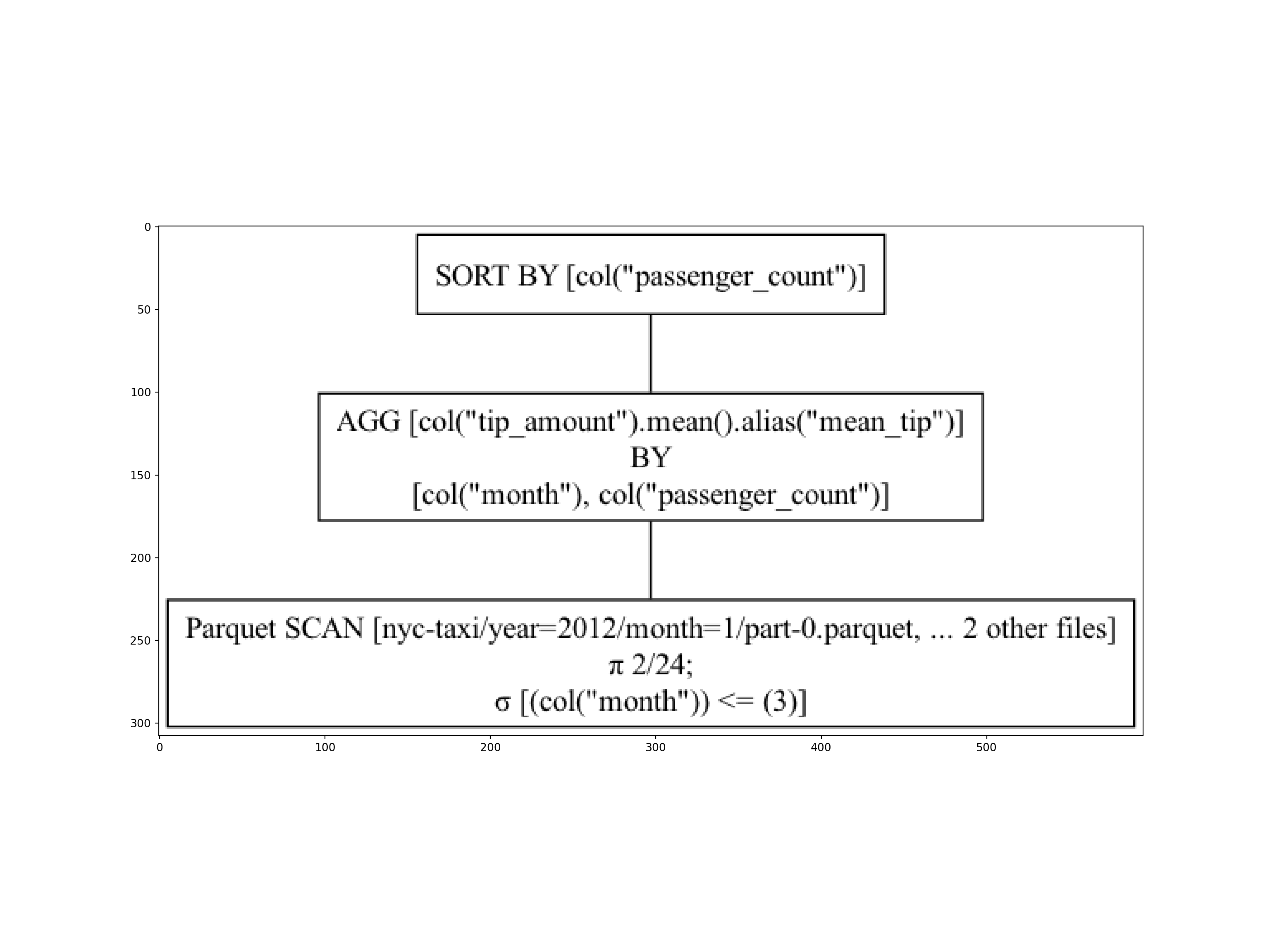
# q2              # naive
cat(q2$explain()) # optimized
SORT BY [col("passenger_count")]
AGGREGATE[maintain_order: false]
[col("tip_amount").mean().alias("mean_tip")] BY [col("month"), col("passenger_count")]
FROM
Parquet SCAN [nyc-taxi/year=2012/month=1/part-0.parquet, ... 2 other sources]
PROJECT 3/24 COLUMNS
SELECTION: [(col("month").cast(Float64)) <= (3.0)]
ESTIMATED ROWS: 44907396Now, let’s run the query and collect the results.
tic = time.time()
dat2 = q2.collect()
toc = time.time()

dat2
shape: (29, 3)
| month | passenger_count | mean_tip |
|---|---|---|
| i64 | i64 | f64 |
| 2 | 0 | 0.876637 |
| 3 | 0 | 0.877675 |
| 1 | 0 | 0.841718 |
| 3 | 1 | 1.089205 |
| 1 | 1 | 1.036863 |
| … | … | … |
| 1 | 9 | 0.0 |
| 2 | 9 | 0.0 |
| 1 | 65 | 0.0 |
| 3 | 208 | 0.0 |
| 1 | 208 | 0.0 |
# print(f"Time difference of {toc - tic} seconds")tic = Sys.time()
dat2 = q2$collect()
toc = Sys.time()
dat2
shape: (29, 3)
| month | passenger_count | mean_tip |
|---|---|---|
| i64 | i64 | f64 |
| 1 | 0 | 0.841718 |
| 2 | 0 | 0.876637 |
| 3 | 0 | 0.877675 |
| 1 | 1 | 1.036863 |
| 2 | 1 | 1.06849 |
| … | … | … |
| 1 | 9 | 0.0 |
| 2 | 9 | 0.0 |
| 1 | 65 | 0.0 |
| 3 | 208 | 0.0 |
| 1 | 208 | 0.0 |
toc - ticTime difference of 0.481447 secsHigh-dimensional grouping example. (Note: this used to provide an example where polars was noticeably slower than DuckDB, but they’ve managed to solve this difference with recent releases.)
q3 = (
    nyc
    .group_by(["passenger_count", "trip_distance"])
    .agg([
        pl.mean("tip_amount").alias("mean_tip"),
        pl.mean("fare_amount").alias("mean_fare"),
        ])
    .sort(["passenger_count", "trip_distance"])
)

tic = time.time()
dat3 = q3.collect()
toc = time.time()

dat3
shape: (25_569, 4)
| passenger_count | trip_distance | mean_tip | mean_fare |
|---|---|---|---|
| i64 | f64 | f64 | f64 |
| 0 | 0.0 | 1.345135 | 17.504564 |
| 0 | 0.01 | 0.178571 | 34.642857 |
| 0 | 0.02 | 4.35 | 61.05 |
| 0 | 0.03 | 16.25 | 74.0 |
| 0 | 0.04 | 0.03 | 46.5 |
| … | … | … | … |
| 208 | 5.1 | 0.0 | 12.5 |
| 208 | 6.6 | 0.0 | 17.7 |
| 247 | 3.31 | 2.3 | 11.5 |
| 249 | 1.69 | 0.0 | 8.5 |
| 254 | 1.02 | 0.0 | 6.0 |
# print(f"Time difference of {toc - tic} seconds")q3 = (
nyc
$group_by("passenger_count", "trip_distance")
$agg(
pl$col("tip_amount")$mean()$alias("mean_tip"),
pl$col("fare_amount")$mean()$alias("mean_fare")
)
$sort("passenger_count", "trip_distance")
)
tic = Sys.time()
dat3 = q3$collect()
toc = Sys.time()
dat3
shape: (25_569, 4)
| passenger_count | trip_distance | mean_tip | mean_fare |
|---|---|---|---|
| i64 | f64 | f64 | f64 |
| 0 | 0.0 | 1.345135 | 17.504564 |
| 0 | 0.01 | 0.178571 | 34.642857 |
| 0 | 0.02 | 4.35 | 61.05 |
| 0 | 0.03 | 16.25 | 74.0 |
| 0 | 0.04 | 0.03 | 46.5 |
| … | … | … | … |
| 208 | 5.1 | 0.0 | 12.5 |
| 208 | 6.6 | 0.0 | 17.7 |
| 247 | 3.31 | 2.3 | 11.5 |
| 249 | 1.69 | 0.0 | 8.5 |
| 254 | 1.02 | 0.0 | 6.0 |
toc - ticTime difference of 5.161533 secsAs an aside, if we didn’t care about column aliases (or sorting), then the previous query could be shortened to:
(
    nyc
    .group_by(["passenger_count", "trip_distance"])
    .agg(pl.col(["tip_amount", "fare_amount"]).mean())
    .collect()
)
(
nyc
$group_by("passenger_count", "trip_distance")
$agg(pl$col("tip_amount", "fare_amount")$mean())
$collect()
)Pivot (reshape)
In polars, we have two distinct reshape methods:
pivot: => long to wideunpivot: => wide to long
Here we’ll unpivot to go from wide to long and use the eager execution engine (i.e., on the dat3 DataFrame object that we’ve already computed) for expediency.
dat3.unpivot(index = ["passenger_count", "trip_distance"])
shape: (51_138, 4)
| passenger_count | trip_distance | variable | value |
|---|---|---|---|
| i64 | f64 | str | f64 |
| 0 | 0.0 | "mean_tip" | 1.345135 |
| 0 | 0.01 | "mean_tip" | 0.178571 |
| 0 | 0.02 | "mean_tip" | 4.35 |
| 0 | 0.03 | "mean_tip" | 16.25 |
| 0 | 0.04 | "mean_tip" | 0.03 |
| … | … | … | … |
| 208 | 5.1 | "mean_fare" | 12.5 |
| 208 | 6.6 | "mean_fare" | 17.7 |
| 247 | 3.31 | "mean_fare" | 11.5 |
| 249 | 1.69 | "mean_fare" | 8.5 |
| 254 | 1.02 | "mean_fare" | 6.0 |
dat3$unpivot(index = c("passenger_count", "trip_distance"))
shape: (51_138, 4)
| passenger_count | trip_distance | variable | value |
|---|---|---|---|
| i64 | f64 | str | f64 |
| 0 | 0.0 | "mean_tip" | 1.345135 |
| 0 | 0.01 | "mean_tip" | 0.178571 |
| 0 | 0.02 | "mean_tip" | 4.35 |
| 0 | 0.03 | "mean_tip" | 16.25 |
| 0 | 0.04 | "mean_tip" | 0.03 |
| … | … | … | … |
| 208 | 5.1 | "mean_fare" | 12.5 |
| 208 | 6.6 | "mean_fare" | 17.7 |
| 247 | 3.31 | "mean_fare" | 11.5 |
| 249 | 1.69 | "mean_fare" | 8.5 |
| 254 | 1.02 | "mean_fare" | 6.0 |
Joins (merges)
mean_tips  = nyc.group_by("month").agg(pl.col("tip_amount").mean())
mean_fares = nyc.group_by("month").agg(pl.col("fare_amount").mean())
(
mean_tips
.join(
mean_fares,
on = "month",
how = "left" # default is inner join
)
.collect()
)
shape: (12, 3)
| month | tip_amount | fare_amount |
|---|---|---|
| i64 | f64 | f64 |
| 3 | 1.056353 | 10.223107 |
| 7 | 1.059312 | 10.379943 |
| 9 | 1.254601 | 12.391198 |
| 1 | 1.007817 | 9.813488 |
| 2 | 1.036874 | 9.94264 |
| … | … | … |
| 6 | 1.091082 | 10.548651 |
| 11 | 1.250903 | 12.270138 |
| 12 | 1.237651 | 12.313953 |
| 8 | 1.079521 | 10.49265 |
| 4 | 1.043167 | 10.33549 |
mean_tips  = nyc$group_by("month")$agg(pl$col("tip_amount")$mean())
mean_fares = nyc$group_by("month")$agg(pl$col("fare_amount")$mean())
(
mean_tips
$join(
mean_fares,
on = "month",
how = "left" # default is inner join
)
$collect()
)
shape: (12, 3)
| month | tip_amount | fare_amount |
|---|---|---|
| i64 | f64 | f64 |
| 1 | 1.007817 | 9.813488 |
| 10 | 1.281239 | 12.501252 |
| 8 | 1.079521 | 10.49265 |
| 11 | 1.250903 | 12.270138 |
| 3 | 1.056353 | 10.223107 |
| … | … | … |
| 12 | 1.237651 | 12.313953 |
| 2 | 1.036874 | 9.94264 |
| 6 | 1.091082 | 10.548651 |
| 9 | 1.254601 | 12.391198 |
| 4 | 1.043167 | 10.33549 |
Appendix: Alternate interfaces
The native polars API is not the only way to interface with the underlying computation engine. Here are two alternate approaches that you may prefer, especially if you don’t want to learn a new syntax.
Ibis (Python)
The great advantage of Ibis (like dbplyr) is that it supports multiple backends through an identical frontend. So, all of our syntax logic and workflow from the Ibis+DuckDB section carry over to an equivalent Ibis+Polars workflow too. All you need to do is change the connection type. For example:
import ibis
import ibis.selectors as s
from ibis import _

##! This next line is the only thing that's changed !##
con = ibis.polars.connect()

nyc = con.read_parquet("nyc-taxi/**/*.parquet")

(
  nyc
  .group_by(["passenger_count"])
  .agg(mean_tip = _.tip_amount.mean())
  .to_polars()
)
shape: (18, 2)
┌─────────────────┬──────────┐
│ passenger_count ┆ mean_tip │
│ --- ┆ --- │
│ i64 ┆ f64 │
╞═════════════════╪══════════╡
│ 9 ┆ 0.8068 │
│ 4 ┆ 0.844519 │
│ 66 ┆ 1.5 │
│ 6 ┆ 1.128365 │
│ 10 ┆ 0.0 │
│ … ┆ … │
│ 7 ┆ 0.544118 │
│ 177 ┆ 1.0 │
│ 208 ┆ 0.0 │
│ 65 ┆ 0.0 │
│ 249 ┆ 0.0 │
└─────────────────┴──────────┘con.disconnect()tidypolars (R)
The R package tidypolars (link) provides the “tidyverse” syntax while using polars as backend. The syntax and workflow should thus be immediately familar to R users.
It’s important to note that tidypolars is solely focused on the translation work. This means that you still need to load the main polars library alongside it for the actual computation, as well as dplyr (and potentially tidyr) for function generics.
library(polars) ## Already loaded
library(tidypolars)
library(dplyr, warn.conflicts = FALSE)
library(tidyr, warn.conflicts = FALSE)

nyc = scan_parquet_polars("nyc-taxi/**/*.parquet")

nyc |>
    summarise(mean_tip = mean(tip_amount), .by = passenger_count) |>
    compute()
shape: (18, 2)
| passenger_count | mean_tip |
|---|---|
| i64 | f64 |
| 0 | 0.862099 |
| 3 | 0.962949 |
| 9 | 0.8068 |
| 6 | 1.128365 |
| 66 | 1.5 |
| … | … |
| 5 | 1.102732 |
| 8 | 0.350769 |
| 65 | 0.0 |
| 208 | 0.0 |
| 247 | 2.3 |
Aside: Use collect() instead of compute() at the end if you would prefer to return a standard R data.frame instead of a Polars DataFrame.
See also polarssql (link) if you would like yet another “tidyverse”-esque alternative that works through DBI/d(b)plyr.