Climate capers at Cato

NOTE: The code and data used to produce all of the figures in this post can be found here.

Having forsworn blogging activity for several months in favour of actual dissertation work, I thought I’d mark a return in time for the holidays. Our topic for discussion today is a poster by Cato Institute researchers, Patrick Michaels and “Chip” Knappenberger.

Michaels & Knappenberger (hereafter M&K) argue that climate models have predicted more warming than we have observed in the global temperature data. It should be noted in passing that this is not a particularly new claim and I may have more to say about the general subject in a future post. Back to the specific matter at hand, however, M&K go further by trying to quantify the mismatch within a formal regression framework. In so doing, they conclude that it is incumbent upon the scientific community to reject current climate models in favour of less “alarmist” ones. (Shots fired!)

Let’s take closer look at their analysis, shall we?

In essence, M&K have implemented a simple linear regression of temperature on a time trend,

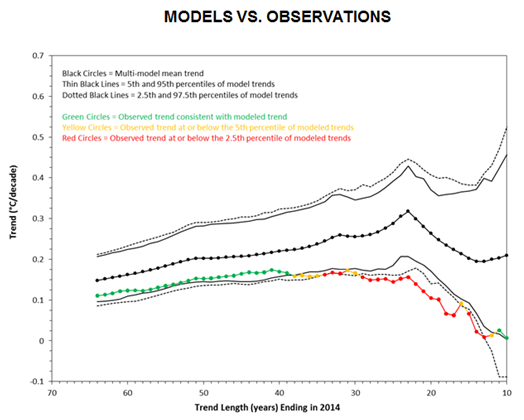
\[Temp_t = \alpha_0 + \beta_1 Trend + \epsilon_t.\]

This is done recursively, starting from 2014 and incrementing backwards one year at a time until the sample extends to the middle of the 20th century. The key figure in their study is shown below and compares the estimated trend coefficient, $\hat{\beta_1}$, from a bunch of climate models (i.e. the CMIP5 ensemble) with that obtained from observed global temperatures (i.e. the UK Met Office’s HadCRUT4 dataset).

Since the observed warming trend consistently falls below that predicted by the suite of climate models, M&K conclude:

“[A]t the global scale, this suite of climate models has failed. Treating them as mathematical hypotheses, which they are, means that it is the duty of scientists to reject their predictions in lieu of those with a lower climate sensitivity.”

These are bold words. Unfortunately for M&K, however, not so bold on substance. As we’re about to see, their analysis is curiously incomplete and their claims begin to unravel under further scrutiny.

Problem 1: Missing confidence intervals

For starters, M&K’s claim about “failed hypotheses” doesn’t make much sense because they haven’t done any actual hypothesis testing. Indeed, they have completely neglected to display confidence intervals. Either that, or (and I’m not sure which is worse) they have forgotten to calculate them in the first place.

The point about missing confidence intervals is really important. The “spread” that we see in the above graph is just a pseudo-interval generated by the full CMIP5 ensemble (i.e. the individual trend means across all 100-odd climate models). It is a measure of model uncertainty, not statistical uncertainty. In other words, we haven’t yet said anything about the confidence intervals attached to each trend estimate, $\hat{\beta_1}$. And, as any first-year econometrics student will tell you, regression coefficients must come with standard errors and corresponding confidence intervals. You could even go so far as to say that accounting for these uncertainties is the very thing that defines hypothesis testing. Can we confidently rule out that a parameter of interest doesn’t overlap with some value or range? Absent these measures of statistical uncertainty, one simply cannot talk meaningfully about a “failed hypothesis”.

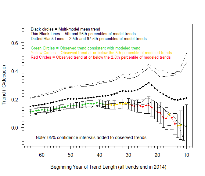
With this mind, I have reproduced the key figure from M&K’s poster, but now with 95% error bars attached to each of the “observed” HadCRUT4 trend estimates. As we can see from the updated graph, the error bars comfortably overlap the model ensemble at every point in time. In fact, the true degree of overlap is even greater than what see in this new figure. That’s because the figure only depicts the error bars which are attached to the trend in observed temperatures. Recall that we are also running the same regression on all 106 climate model. Each of these regressions will produce a trend estimate with its own error bars. This will widen the ensemble range and further underscore the degree of overlap between the models and observations. (Again, with the computer models we have to account for both the spread between the models’ mean coefficient estimates and their associated individual standard errors. This is one reason why this type of regression exercise is fairly limited – it doubles up on uncertainty.) Whatever the case, it seems fair to say that M&K’s bold assertion that we need to reject the climate models as “failed hypotheses” simply does not hold water.

Problem 2: Fixed starting date

My second problem with M&K’s approach is their choice of a recursive regression model and fixed starting point. The starting point for all of the individual regressions is 2014, which just happens to be a year where observed temperatures were unusually low compared to the model estimates; at least, relative to other years. In other words, M&K are anchoring their results in a way that distorts the relative trends along the remainder of the recursive series.

Now, you may counter that it makes sense to use the most recent year as your starting point. However, the principle remains: Privileging observations from any particular year is going to give you misleading results in climate research, where the long-term is what really matters. This problem is exacerbated in the present case, because of the aforementioned absence of confidence intervals. The early discrepancies between the models and observations have to be discounted because that is where the confidence intervals are largest (due to the smaller sample size). And, yet, you would have no idea that this was a problem if you only looked at M&K’s original figure. Again, the missing confidence intervals gives the misleading impression that all points are “created equal”, when they simply aren’t from a statistical perspective.

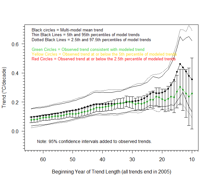
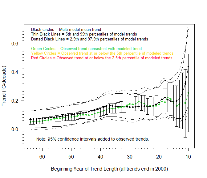
Rather than a recursive regression, I would therefore argue that a rolling regression offers a much better way of investigating the performance of climate models. Another alternative is to stick with recursive regressions, but to vary the starting date. This is what I have done in the figures below, using 2005 and then 2000 as the new fixed points. (For the sake of comparison, I keep the maximum trend length the same, so each of these figures goes a little further back in time.) The effect on the relative trend slopes – and therefore the agreement between climate models and observations – is clear to see.