Draw coefficient plots and interaction plots from fixest regression objects.
Source: R/ggcoefplot.R, R/ggiplot.R
ggcoefplot.RdDraws the ggplot2 equivalents of fixest::coefplot and
fixest::iplot. These "gg*" versions do their best to recycle the same
arguments and plotting logic as their original base counterparts. But they
also support additional features via the ggplot2 API and infrastructure.
The overall goal remains the same as the original functions. To wit:
ggcoefplot plots the results of estimations (coefficients and confidence
intervals). The function ggiplot restricts the output to variables
created with i, either interactions with factors or raw factors.
Usage
ggcoefplot(
  object,
  geom_style = c("pointrange", "errorbar"),
  multi_style = c("dodge", "facet"),
  facet_args = NULL,
  theme = NULL,
  ...
)

ggiplot(
  object,
  geom_style = c("pointrange", "errorbar", "ribbon"),
  multi_style = c("dodge", "facet"),
  aggr_eff = NULL,
  aggr_eff.par = list(col = "gray", lwd = 1, lty = 1),
  facet_args = NULL,
  theme = NULL,
  ...
)
Arguments
- object
A model object of class
fixestorfixest_multi, or a list thereof.- geom_style
Character string. One of
c('pointrange', 'errorbar', 'ribbon')describing the preferred geometric representation of the coefficients. Note that ribbon plots not supported forggcoefplot, since we cannot guarantee a continuous relationship among the coefficients.- multi_style
Character string. One of
c('dodge', 'facet'), defining how multi-model objects should be presented.- facet_args
A list of arguments passed down to
ggplot::fact_wrap(). E.g.facet_args = list(ncol = 2, scales = 'free_y'). Only used ifmulti_style = 'facet'.- theme
ggplot2 theme. Defaults to
theme_linedraw()with some minor adjustments, such as centered plot title. Can also be defined on an existing ggiplot object to redefine theme elements. See examples.- ...
Arguments passed down to, or equivalent to, the corresponding
fixest::coefplot/fixest::iplotarguments. Note that some of these require list objects. Currently used are:keepanddropfor subsetting variables using regular expressions. Thefixest::iplothelp page includes more detailed examples, but these should generally work as you expect. One useful regexp trick worth mentioning briefly for event studies with many pre-/post-periods isdrop = "[[:digit:]]{2}". This will cause the plot to zoom in around single digit pre-/post-periods.groupa list indicating variables to group over. Each element of the list reports the coefficients to be grouped while the name of the element is the group name. Each element of the list can be either: i) a character vector of length 1, ii) of length 2, or iii) a numeric vector. Special patterns such as "^^var_start" can be used to more appealing plotting, where group labels are separated from their subsidiary labels. This can be especially useful for plotting interaction terms. See the Details section offixest::coefplotfor more information.i.selectInteger scalar, default is 1. Inggiplot, used to select which variable created withi()to select. Only used when there are several variables created withi. See the Details section offixest::iplotfor more information.main,xlab, andylabfor setting the plot title, x- and y-axis labels, respectively.zeroandzero.parfor defining or adjusting the zero line. For example,zero.par = list(col = 'orange').ref.lineandref.line.parfor defining or adjusting the vertical reference line. For example,ref.line.par = list(col = 'red', lty = 4).pt.pchandpt.joinfor overriding the default point estimate shapes and joining them, respectively.colfor manually defining line, point, and ribbon colours.ci_levelfor changing the desired confidence level (default = 0.95). Note that multiple levels are allowed, e.g.ci_level = c(0.8, 0.95).ci.widthfor changing the width of the extremities of the confidence intervals. Only used ifgeom_style = "errorbar"(or if multiple CI levels are requested for the default pointrange style). The default value is 0.2.ci.fill.parfor changing the confidence interval fill. Only used whengeom_style = "ribbon"and currently only affects the alpha (transparency) channel. For example, we can make the CI band lighter withci.fill.par = list(alpha = 0.2)(the default alpha is 0.3).dicta dictionary for overriding coefficient names.vcov,clusterorseas alternative options for adjusting the standard errors of the model object(s) on the fly. Seevcov.fixestfor details. Written here in superseding order;clusterwill only be considered ifvcovis not null, etc.
- aggr_eff
A keyword string or numeric sequence, indicating whether mean treatment effects for some subset of the model should be displayed as part of the plot. For example, the
"post"keyword means that the mean post-treatment effect will be plotted alongside the individual period effects. Passed toaggr_es; see that function's documentation for other valid options.- aggr_eff.par
List. Parameters of the aggregated treatment effect line, if plotted. The default values are
col = 'gray',lwd = 1,lty = 1.
Details
These functions generally try to mimic the functionality and (where
appropriate) arguments of fixest::coefplot and fixest::iplot as
closely as possible. However, by leveraging the ggplot2 API and
infrastructure, they are able to support some more complex plot
arrangements out-of-the-box that would be more difficult to achieve using
the base coefplot/iplot alternatives.
Functions
ggiplot(): This function plots the results of estimations (coefficients and confidence intervals). The functionggiplotrestricts the output to variables created with i, either interactions with factors or raw factors.
Examples
library(ggfixest)
##
# Author note: The examples that follow deliberately follow the original
# examples from the coefplot/iplot help pages. A few "gg-" specific
# features are sprinkled within, with the final set of examples in
# particular highlighting unique features of this package.
#
# Example 1: Basic use and stacking two sets of results on the same graph
#
# Estimation on Iris data with one fixed-effect (Species)
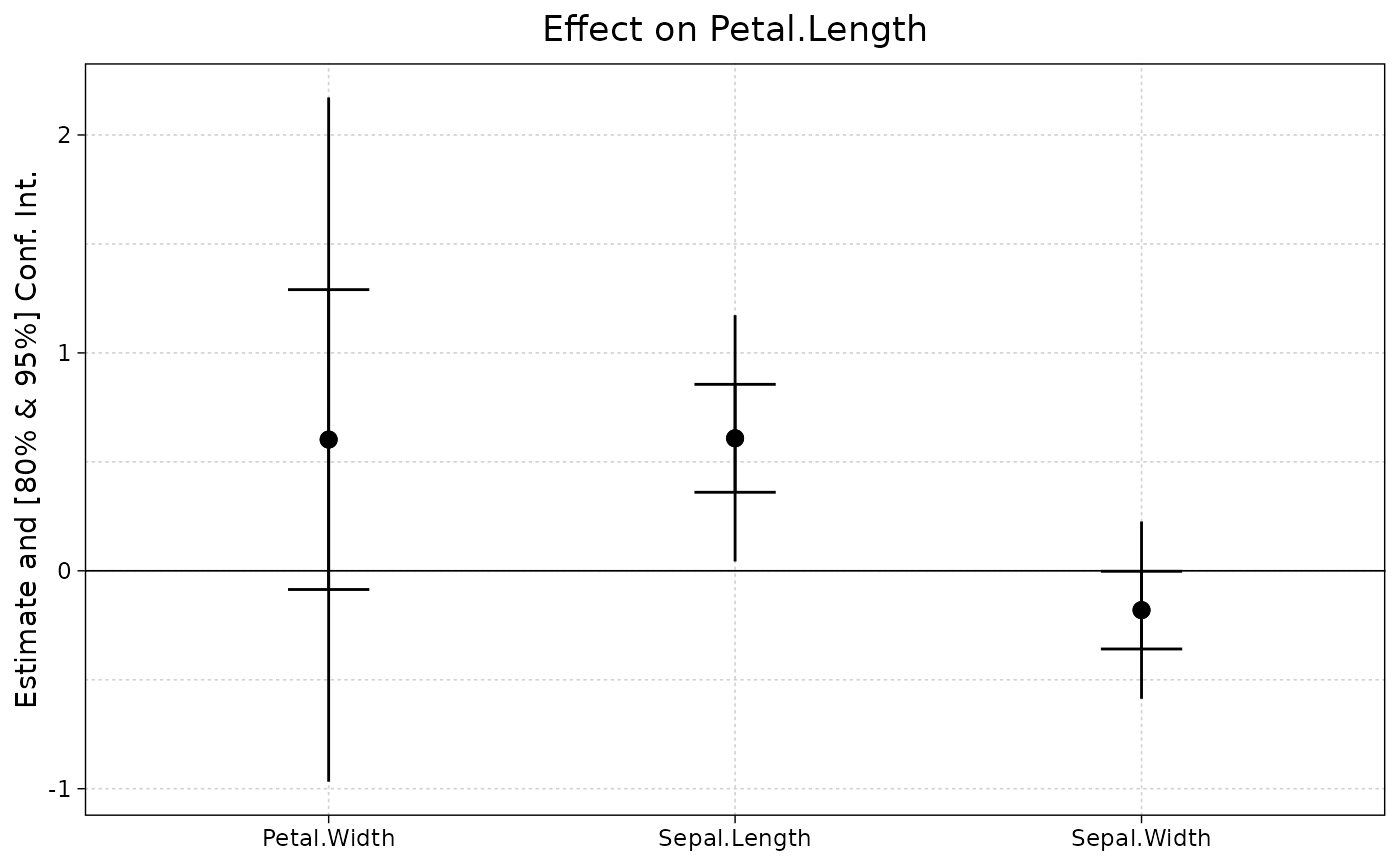
est = feols(Petal.Length ~ Petal.Width + Sepal.Length + Sepal.Width | Species, iris)
ggcoefplot(est)
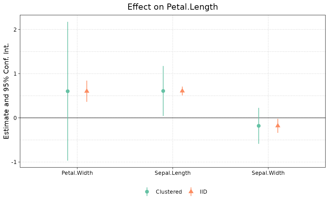
 # Add/compare multiple SE types on the fly
ggcoefplot(est, vcov = list("iid", "hc1"))
# Add/compare multiple SE types on the fly
ggcoefplot(est, vcov = list("iid", "hc1"))
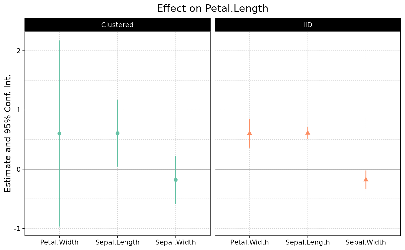
 # ... or as separate facets
ggcoefplot(est, vcov = list("iid", "hc1"), multi_style = "facet") +
theme(legend.position = "none")
# ... or as separate facets
ggcoefplot(est, vcov = list("iid", "hc1"), multi_style = "facet") +
theme(legend.position = "none")
 # Show multiple CIs
ggcoefplot(est, ci_level = c(0.8, 0.95))
# Show multiple CIs
ggcoefplot(est, ci_level = c(0.8, 0.95))
 # Combine multiple CIs with multiple SE types
ggcoefplot(est, ci_level = c(0.8, 0.95), vcov = list("iid", "hc1"))
# Combine multiple CIs with multiple SE types
ggcoefplot(est, ci_level = c(0.8, 0.95), vcov = list("iid", "hc1"))
 #
#
# Example 2: Interactions
#
# Now we estimate and plot the "yearly" treatment effects
data(base_did)
base_inter = base_did
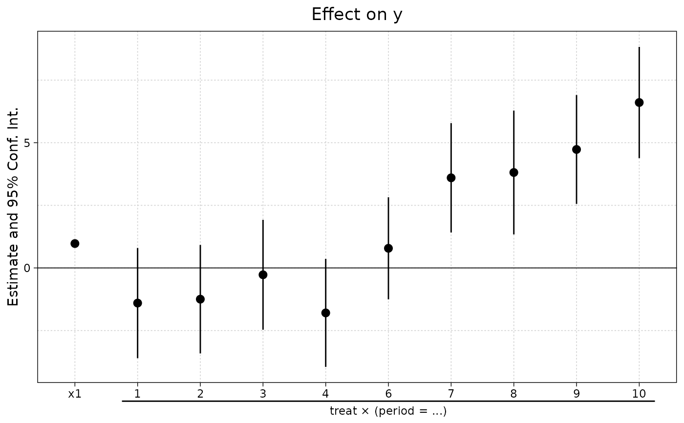
# We interact the variable 'period' with the variable 'treat'
est_did = feols(y ~ x1 + i(period, treat, 5) | id + period, base_inter,
vcov = ~id)
# In the estimation, the variable treat is interacted
# with each value of period but 5, set as a reference
# ggcoefplot will show all the coefficients:
ggcoefplot(est_did)
#
#
# Example 2: Interactions
#
# Now we estimate and plot the "yearly" treatment effects
data(base_did)
base_inter = base_did
# We interact the variable 'period' with the variable 'treat'
est_did = feols(y ~ x1 + i(period, treat, 5) | id + period, base_inter,
vcov = ~id)
# In the estimation, the variable treat is interacted
# with each value of period but 5, set as a reference
# ggcoefplot will show all the coefficients:
ggcoefplot(est_did)
 # Note that the grouping of the coefficients is due to 'group = "auto"'
# If you want to keep only the coefficients
# created with i() (ie the interactions), use ggiplot
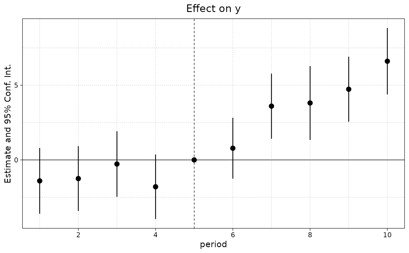
ggiplot(est_did)
# Note that the grouping of the coefficients is due to 'group = "auto"'
# If you want to keep only the coefficients
# created with i() (ie the interactions), use ggiplot
ggiplot(est_did)
 # We can see that the graph is different from before:
# - only interactions are shown,
# - the reference is present,
# => this is fully flexible
ggiplot(est_did, ci_level = c(0.8, 0.95))
# We can see that the graph is different from before:
# - only interactions are shown,
# - the reference is present,
# => this is fully flexible
ggiplot(est_did, ci_level = c(0.8, 0.95))
 ggiplot(est_did, ref.line = FALSE, pt.join = TRUE, geom_style = "errorbar")
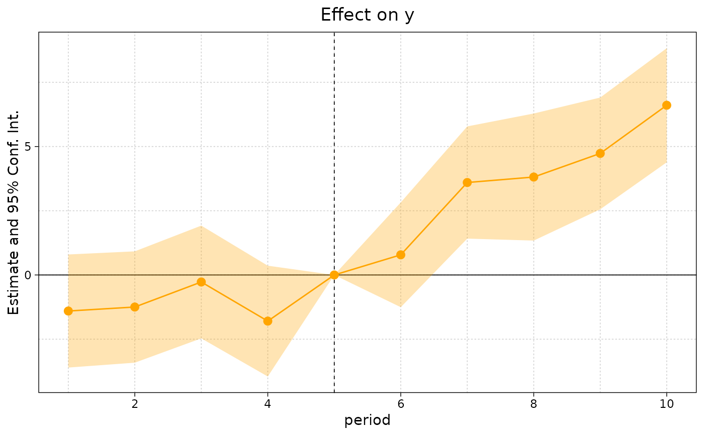 ggiplot(est_did, geom_style = "ribbon", col = "hotpink")
#> Scale for colour is already present.
#> Adding another scale for colour, which will replace the existing scale.
ggiplot(est_did, geom_style = "ribbon", col = "hotpink")
#> Scale for colour is already present.
#> Adding another scale for colour, which will replace the existing scale.
 ggiplot(est_did, aggr_eff = "both")
 # etc
# We can also use a dictionary to replace label values. The dicionary should
# take the form of a named vector or list, e.g. c("old_lab1" = "new_lab1", ...)
# Let's create a "month" variable
all_months = c("aug", "sept", "oct", "nov", "dec", "jan",
"feb", "mar", "apr", "may", "jun", "jul")
# Turn into a dictionary by providing the old names
# Note the implication that treatment occured here in December (5 month in our series)
dict = all_months; names(dict) = 1:12
# Pass our new dictionary to our ggiplot call
ggiplot(est_did, pt.join = TRUE, geom_style = "errorbar", dict = dict)
# etc
# We can also use a dictionary to replace label values. The dicionary should
# take the form of a named vector or list, e.g. c("old_lab1" = "new_lab1", ...)
# Let's create a "month" variable
all_months = c("aug", "sept", "oct", "nov", "dec", "jan",
"feb", "mar", "apr", "may", "jun", "jul")
# Turn into a dictionary by providing the old names
# Note the implication that treatment occured here in December (5 month in our series)
dict = all_months; names(dict) = 1:12
# Pass our new dictionary to our ggiplot call
ggiplot(est_did, pt.join = TRUE, geom_style = "errorbar", dict = dict)
 #
# What if the interacted variable is not numeric? (tl;dr use a factor)
# let's re-use our all_months vector from the previous example, but add it
# directly to the dataset
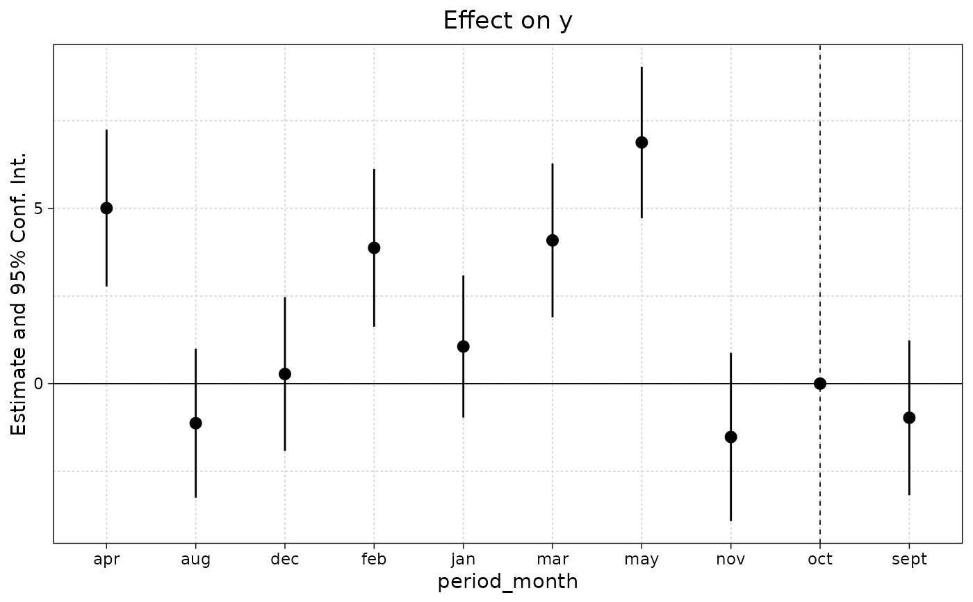
base_inter$period_month = all_months[base_inter$period]
# NB: Since 'period_month' of type character, iplot/coefplot both sort it
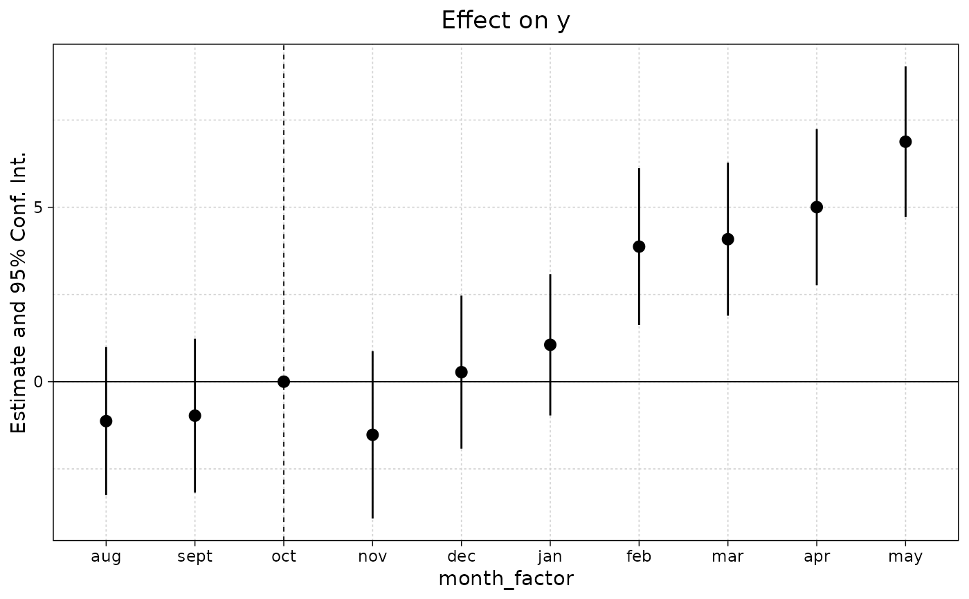
# alphabetically... To respect a plotting order, rather use a factor
base_inter$month_factor = factor(base_inter$period_month, levels = all_months)
est = feols(y ~ x1 + i(month_factor, treat, "oct") | id + period, base_inter,
vcov = ~id)
ggiplot(est)
#
# What if the interacted variable is not numeric? (tl;dr use a factor)
# let's re-use our all_months vector from the previous example, but add it
# directly to the dataset
base_inter$period_month = all_months[base_inter$period]
# NB: Since 'period_month' of type character, iplot/coefplot both sort it
# alphabetically... To respect a plotting order, rather use a factor
base_inter$month_factor = factor(base_inter$period_month, levels = all_months)
est = feols(y ~ x1 + i(month_factor, treat, "oct") | id + period, base_inter,
vcov = ~id)
ggiplot(est)
 # dict -> c("old_name" = "new_name")
dict = all_months; names(dict) = 1:12; dict
#> 1 2 3 4 5 6 7 8 9 10 11
#> "aug" "sept" "oct" "nov" "dec" "jan" "feb" "mar" "apr" "may" "jun"
#> 12
#> "jul"
ggiplot(est_did, dict = dict)
# dict -> c("old_name" = "new_name")
dict = all_months; names(dict) = 1:12; dict
#> 1 2 3 4 5 6 7 8 9 10 11
#> "aug" "sept" "oct" "nov" "dec" "jan" "feb" "mar" "apr" "may" "jun"
#> 12
#> "jul"
ggiplot(est_did, dict = dict)
 #
# Example 3: Setting defaults
#
# The customization logic of ggcoefplot/ggiplot works differently than the
# original base fixest counterparts, so we don't have "gg" equivalents of
# setFixest_coefplot and setFixest_iplot. However, you can still invoke some
# global fixest settings like setFixest_dict(). SImple example:
base_inter$letter = letters[base_inter$period]
est_letters = feols(y ~ x1 + i(letter, treat, 'e') | id + letter, base_inter,
vcov = ~id)
# Set global dictionary for capitalising the letters
dict = LETTERS[1:10]; names(dict) = letters[1:10]
setFixest_dict(dict)
ggiplot(est_letters)
#
# Example 3: Setting defaults
#
# The customization logic of ggcoefplot/ggiplot works differently than the
# original base fixest counterparts, so we don't have "gg" equivalents of
# setFixest_coefplot and setFixest_iplot. However, you can still invoke some
# global fixest settings like setFixest_dict(). SImple example:
base_inter$letter = letters[base_inter$period]
est_letters = feols(y ~ x1 + i(letter, treat, 'e') | id + letter, base_inter,
vcov = ~id)
# Set global dictionary for capitalising the letters
dict = LETTERS[1:10]; names(dict) = letters[1:10]
setFixest_dict(dict)
ggiplot(est_letters)
 setFixest_dict() # reset
#
# Example 4: group + cleaning
#
# You can use the argument group to group variables
# You can further use the special character "^^" to clean
# the beginning of the coef. name: particularly useful for factors
est = feols(Petal.Length ~ Petal.Width + Sepal.Length +
Sepal.Width + Species, iris)
# No grouping:
ggcoefplot(est)
setFixest_dict() # reset
#
# Example 4: group + cleaning
#
# You can use the argument group to group variables
# You can further use the special character "^^" to clean
# the beginning of the coef. name: particularly useful for factors
est = feols(Petal.Length ~ Petal.Width + Sepal.Length +
Sepal.Width + Species, iris)
# No grouping:
ggcoefplot(est)
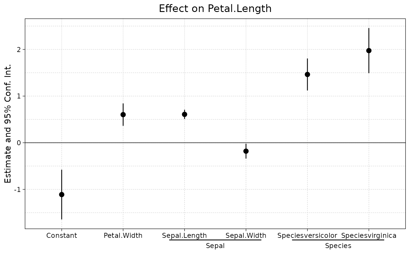 # now we group by Sepal and Species
ggcoefplot(est, group = list(Sepal = "Sepal", Species = "Species"))
# now we group by Sepal and Species
ggcoefplot(est, group = list(Sepal = "Sepal", Species = "Species"))
 # now we group + clean the beginning of the names using the special character ^^
ggcoefplot(est, group = list(Sepal = "^^Sepal.", Species = "^^Species"))
# now we group + clean the beginning of the names using the special character ^^
ggcoefplot(est, group = list(Sepal = "^^Sepal.", Species = "^^Species"))
 #
# Example 5: Some more ggcoefplot/ggiplot extras
#
# We'll demonstrate using the staggered treatment example from the
# introductory fixest vignette.
data(base_stagg)
est_twfe = feols(
y ~ x1 + i(time_to_treatment, treated, ref = c(-1, -1000)) | id + year,
base_stagg,
vcov = ~id
)
est_sa20 = feols(
y ~ x1 + sunab(year_treated, year) | id + year,
data = base_stagg,
vcov = ~id
)
#> Warning: The VCOV matrix is not positive semi-definite and was 'fixed' (see ?vcov).
# Plot both regressions in a faceted plot
ggiplot(
list('TWFE' = est_twfe, 'Sun & Abraham (2020)' = est_sa20),
main = 'Staggered treatment', ref.line = -1, pt.join = TRUE
)
#
# Example 5: Some more ggcoefplot/ggiplot extras
#
# We'll demonstrate using the staggered treatment example from the
# introductory fixest vignette.
data(base_stagg)
est_twfe = feols(
y ~ x1 + i(time_to_treatment, treated, ref = c(-1, -1000)) | id + year,
base_stagg,
vcov = ~id
)
est_sa20 = feols(
y ~ x1 + sunab(year_treated, year) | id + year,
data = base_stagg,
vcov = ~id
)
#> Warning: The VCOV matrix is not positive semi-definite and was 'fixed' (see ?vcov).
# Plot both regressions in a faceted plot
ggiplot(
list('TWFE' = est_twfe, 'Sun & Abraham (2020)' = est_sa20),
main = 'Staggered treatment', ref.line = -1, pt.join = TRUE
)
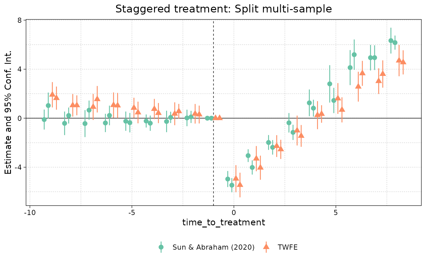 # So far that's no different than base iplot (automatic legend aside). But an
# area where ggiplot shines is in complex multiple estimation cases, such as
# lists of fixest_multi objects. To illustrate, let's add a split variable
# (group) to our staggered dataset.
base_stagg_grp = base_stagg
base_stagg_grp$grp = ifelse(base_stagg_grp$id %% 2 == 0, 'Evens', 'Odds')
# Now re-run our two regressions from earlier, but splitting the sample to
# generate fixest_multi objects.
est_twfe_grp = feols(
y ~ x1 + i(time_to_treatment, treated, ref = c(-1, -1000)) | id + year,
data = base_stagg_grp, split = ~ grp,
vcov = ~id
)
est_sa20_grp = feols(
y ~ x1 + sunab(year_treated, year) | id + year,
data = base_stagg_grp, split = ~ grp,
vcov = ~id
)
#> Warning: The VCOV matrix is not positive semi-definite and was 'fixed' (see ?vcov).
#> Warning: The VCOV matrix is not positive semi-definite and was 'fixed' (see ?vcov).
# ggiplot combines the list of multi-estimation objects without a problem...
ggiplot(list('TWFE' = est_twfe_grp, 'Sun & Abraham (2020)' = est_sa20_grp),
ref.line = -1, main = 'Staggered treatment: Split multi-sample')
# So far that's no different than base iplot (automatic legend aside). But an
# area where ggiplot shines is in complex multiple estimation cases, such as
# lists of fixest_multi objects. To illustrate, let's add a split variable
# (group) to our staggered dataset.
base_stagg_grp = base_stagg
base_stagg_grp$grp = ifelse(base_stagg_grp$id %% 2 == 0, 'Evens', 'Odds')
# Now re-run our two regressions from earlier, but splitting the sample to
# generate fixest_multi objects.
est_twfe_grp = feols(
y ~ x1 + i(time_to_treatment, treated, ref = c(-1, -1000)) | id + year,
data = base_stagg_grp, split = ~ grp,
vcov = ~id
)
est_sa20_grp = feols(
y ~ x1 + sunab(year_treated, year) | id + year,
data = base_stagg_grp, split = ~ grp,
vcov = ~id
)
#> Warning: The VCOV matrix is not positive semi-definite and was 'fixed' (see ?vcov).
#> Warning: The VCOV matrix is not positive semi-definite and was 'fixed' (see ?vcov).
# ggiplot combines the list of multi-estimation objects without a problem...
ggiplot(list('TWFE' = est_twfe_grp, 'Sun & Abraham (2020)' = est_sa20_grp),
ref.line = -1, main = 'Staggered treatment: Split multi-sample')
 # ... but is even better when we use facets instead of dodged errorbars.
# Let's use this an opportunity to construct a fancy plot that invokes some
# additional arguments and ggplot theming.
ggiplot(
list('TWFE' = est_twfe_grp, 'Sun & Abraham (2020)' = est_sa20_grp),
ref.line = -1,
main = 'Staggered treatment: Split multi-sample',
xlab = 'Time to treatment',
multi_style = 'facet',
geom_style = 'ribbon',
facet_args = list(labeller = labeller(id = function(x) gsub(".*: ", "", x))),
theme = theme_minimal() +
theme(
text = element_text(family = 'HersheySans'),
plot.title = element_text(hjust = 0.5),
legend.position = 'none'
)
)
# ... but is even better when we use facets instead of dodged errorbars.
# Let's use this an opportunity to construct a fancy plot that invokes some
# additional arguments and ggplot theming.
ggiplot(
list('TWFE' = est_twfe_grp, 'Sun & Abraham (2020)' = est_sa20_grp),
ref.line = -1,
main = 'Staggered treatment: Split multi-sample',
xlab = 'Time to treatment',
multi_style = 'facet',
geom_style = 'ribbon',
facet_args = list(labeller = labeller(id = function(x) gsub(".*: ", "", x))),
theme = theme_minimal() +
theme(
text = element_text(family = 'HersheySans'),
plot.title = element_text(hjust = 0.5),
legend.position = 'none'
)
)
